
Travel Google Search Trend Prediction#
Business Questions#
Business Question 1: What are the external factors that impact the volume of Google Search about domestic travel to Las Vegas in United State?
Granger Causarity Test
H0: The input variable X does not cause the changes in the future demand of output variable Y.
H1: The input variable X does cause the change in the future demand of output variable Y.
Cointegration Test
Business Question 2: What is the time lag between the external factors impact the volume of Google Search?
Pick the Order (P) of VAR model that gives a model with the least AIC by iteratively fit increasing orders of VAR model
Business Question 3: How to determ the variables to incporate into the demand forecasting model?
Select the best performing model based on Root Mean Squared Error (RMSE), Mean Absolute Percentage Error (MAPE), Mean Absolute Error (MAE), and Mean Squared Error (MSE)
import pandas as pd
import numpy as np
import matplotlib.pyplot as plt
%matplotlib inline
import seaborn as sns
from datetime import datetime

# Import Statsmodels
from statsmodels.tsa.api import VAR
from statsmodels.tsa.stattools import adfuller
from statsmodels.tools.eval_measures import rmse, aic

#supress scientific notation
pd.set_option('display.float_format', '{:.3f}'.format)
To-Dos#
Import the dataset
Analyze the time series characteristics
Test for causation among the time series
Test for cointegration among the time series
Split the dataset into Training and Test
Test for stationarity
Transform the series to make it stationary, if needed
Find optimal order (p)
Prepare training and test datasets
Train the model
Roll back the transformations, if any.
Evaluate the model using test set
Forecast to future
1. Import the dataset#
df = pd.read_csv('travel_data.csv', parse_dates=True)
df = df.sort_values('DATE').reset_index(drop=True)
df = df[df['DATE']>='2018']
df['Visitor Volume'] = df['Visitor Volume'].astype('int')
df['DATE'] = pd.to_datetime(df['DATE']).dt.strftime('%Y-%m')
df.set_index('DATE', inplace = True)
df.index = pd.DatetimeIndex(df.index, freq=None)

df.tail()
| Google Trend Index | Visitor Volume | Average Daily Room Rate (ADR) | CPI | Unemployment Rate | Cost per Gallon | |
|---|---|---|---|---|---|---|
| DATE | ||||||
| 2023-01-01 | 78 | 3275300 | 191.620 | 299.170 | 3.400 | 3.330 |
| 2023-02-01 | 78 | 3081800 | 176.640 | 300.840 | 3.600 | 3.250 |
| 2023-03-01 | 80 | 3655800 | 213.250 | 301.836 | 3.500 | 2.930 |
| 2023-04-01 | 75 | 3385500 | 171.050 | 303.363 | 3.400 | 2.660 |
| 2023-05-01 | 79 | 3498000 | 183.400 | 304.127 | 3.700 | 3.450 |
# Normalize the visitor volume, Average Daily Room Rate, and CPI data with Z-score
avg, dev  = df['Visitor Volume'].mean(), df['Visitor Volume'].std()
df['Visitor Volume'] = (df['Visitor Volume']-avg)/dev

avg, dev  = df['Average Daily Room Rate (ADR)'].mean(), df['Average Daily Room Rate (ADR)'].std()
df['Average Daily Room Rate (ADR)'] = (df['Average Daily Room Rate (ADR)']-avg)/dev

avg, dev  = df['CPI'].mean(), df['CPI'].std()
df['CPI'] = (df['CPI']-avg)/dev

df
| Google Trend Index | Visitor Volume | Average Daily Room Rate (ADR) | CPI | Unemployment Rate | Cost per Gallon | |
|---|---|---|---|---|---|---|
| DATE | ||||||
| 2018-01-01 | 87 | 0.496 | 0.421 | -1.167 | 4.000 | 2.020 |
| 2018-02-01 | 87 | 0.203 | -0.566 | -1.104 | 4.100 | 2.020 |
| 2018-03-01 | 89 | 0.892 | -0.120 | -1.072 | 4.000 | 1.960 |
| 2018-04-01 | 82 | 0.668 | -0.279 | -1.016 | 4.000 | 2.080 |
| 2018-05-01 | 88 | 0.759 | -0.120 | -0.957 | 3.800 | 2.180 |
| ... | ... | ... | ... | ... | ... | ... |
| 2023-01-01 | 78 | 0.364 | 1.714 | 1.719 | 3.400 | 3.330 |
| 2023-02-01 | 78 | 0.149 | 1.237 | 1.813 | 3.600 | 3.250 |
| 2023-03-01 | 80 | 0.787 | 2.402 | 1.869 | 3.500 | 2.930 |
| 2023-04-01 | 75 | 0.487 | 1.059 | 1.955 | 3.400 | 2.660 |
| 2023-05-01 | 79 | 0.612 | 1.452 | 1.998 | 3.700 | 3.450 |
65 rows × 6 columns
#The list of variables
input_variables = df.columns.values[1:].tolist()
input_variables
['Visitor Volume',
 'Average Daily Room Rate (ADR)',
 'CPI',
 'Unemployment Rate',
 'Cost per Gallon']
2. Analyze the characteristics of the time series#
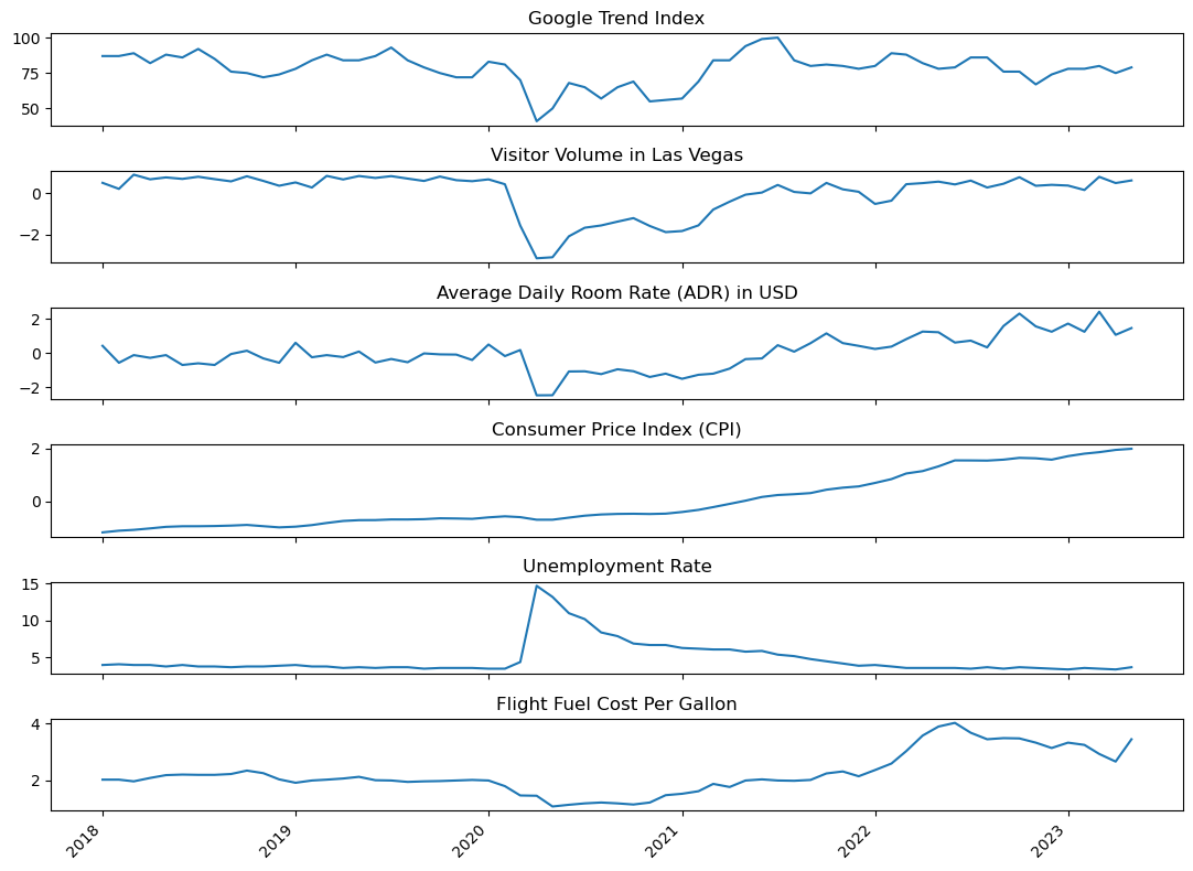
#Visualize the overall trend of each time series

fig, (ax1, ax2, ax3, ax4, ax5, ax6) = plt.subplots(6,1, figsize = (11,8), sharex=True)
ax1.plot(df.index,df['Google Trend Index'])
ax1.set_title('Google Trend Index')

ax2.plot(df.index,df['Visitor Volume'])
ax2.set_title('Visitor Volume in Las Vegas')

ax3.plot(df.index,df['Average Daily Room Rate (ADR)'])
ax3.set_title('Average Daily Room Rate (ADR) in USD')

ax4.plot(df.index, df['CPI'])
ax4.set_title('Consumer Price Index (CPI)')

ax5.plot(df.index, df['Unemployment Rate'])
ax5.set_title('Unemployment Rate')

ax6.plot(df.index, df['Cost per Gallon'])
ax6.set_title('Flight Fuel Cost Per Gallon')

fig.autofmt_xdate(rotation=45)
plt.tight_layout()
;
''
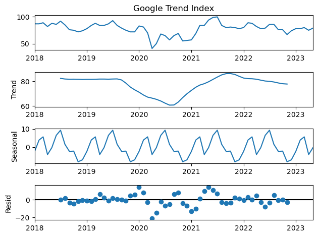
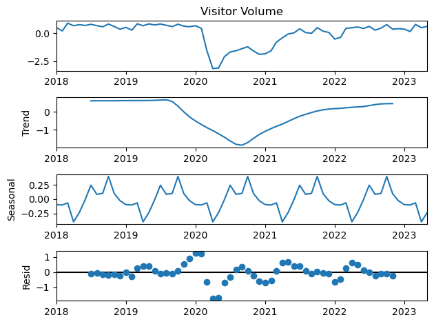
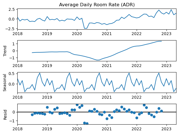
# A function to create Decomposition and plot trend, seasonality, and errors
def decomposition(df):
    from statsmodels.tsa.seasonal import seasonal_decompose
    variables = df.columns.values
    for i in variables:
        result = seasonal_decompose(df[i])

        fig = plt.figure(figsize = (12,8))
        fix = result.plot();
decomposition(df)
<Figure size 1200x800 with 0 Axes>
<Figure size 1200x800 with 0 Axes>
<Figure size 1200x800 with 0 Axes>
<Figure size 1200x800 with 0 Axes>
<Figure size 1200x800 with 0 Axes>
<Figure size 1200x800 with 0 Axes>
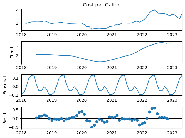
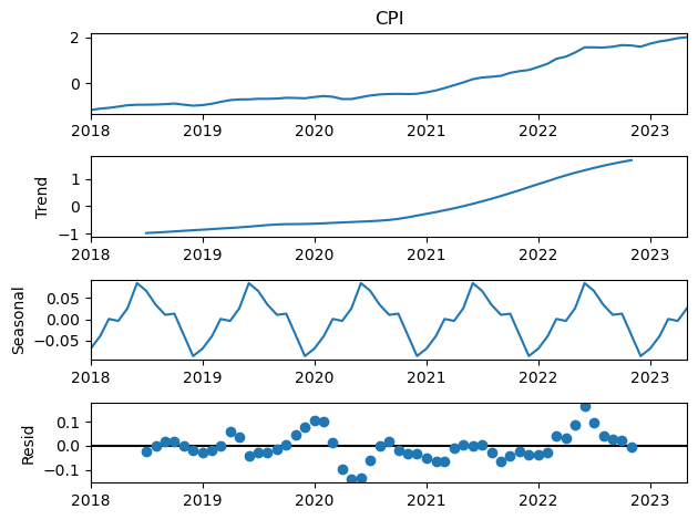
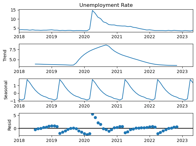
Observations#
Google Trend Index, Visitor voluhme, Verage daily room rate has failry similar trend.
Flight Fuel has somewhat similar trend as Google Trend Index but slighly lagged from the Google Trend index.
Exmplotment rate is an inverse relationship to Google Trend Index
Consumer Price index does not seem to have similar trend as Google Trend Index.
3. Test for Causation using Granger’s Causality Test#
Granger’s Causality Test Null Hypothesis: The past value of input variable X do not cause the output variable Y.
H0: The past value of the input variable X does not cause the output variable Y.
H1: The past value of the input variable X causes the output variable Y.
Row (Y): Output variables
Columns (X): Inputvariables
If s given p-value is < 0.05, the corresponding X series (column) causes the Y (row).
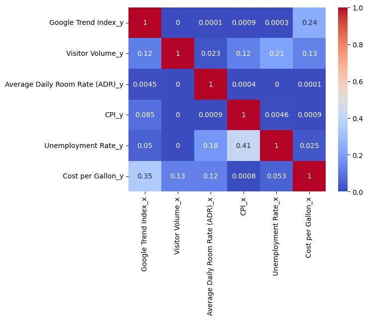
#A funcion to check Granger's causality of all possible combination of the time series
def check_causality(data, variables, test='ssr_chi2test', verbose=False, maxlag = 12):
    from statsmodels.tsa.stattools import grangercausalitytests
    #create a empty DataFram:
        #Columns: variables
        #Rows: Variables
    df = pd.DataFrame(np.zeros((len(variables), len(variables))), columns = variables, index=variables)
    for col in df.columns:
        for row in df.index:
            test_result = grangercausalitytests(data[[row, col]], maxlag=maxlag, verbose=verbose)
            p_values = [round(test_result[i+1][0][test][1],4) for i in range(maxlag)]
            if verbose: print(f'Y = {row}, X = {col}, P Values = {p_values}')
            min_p_value = np.min(p_values)
            df.loc[row, col] = min_p_value
    df.columns = [var + '_x' for var in variables]
    df.index = [var + '_y' for var in variables]

    sns.heatmap(df, cmap='coolwarm', annot= True)

    return df
causality = check_causality(df, df.columns.values)
causality
| Google Trend Index_x | Visitor Volume_x | Average Daily Room Rate (ADR)_x | CPI_x | Unemployment Rate_x | Cost per Gallon_x | |
|---|---|---|---|---|---|---|
| Google Trend Index_y | 1.000 | 0.000 | 0.000 | 0.001 | 0.000 | 0.242 |
| Visitor Volume_y | 0.121 | 1.000 | 0.023 | 0.122 | 0.212 | 0.127 |
| Average Daily Room Rate (ADR)_y | 0.004 | 0.000 | 1.000 | 0.000 | 0.000 | 0.000 |
| CPI_y | 0.085 | 0.000 | 0.001 | 1.000 | 0.005 | 0.001 |
| Unemployment Rate_y | 0.050 | 0.000 | 0.183 | 0.415 | 1.000 | 0.025 |
| Cost per Gallon_y | 0.351 | 0.125 | 0.123 | 0.001 | 0.053 | 1.000 |
causality.to_csv('causality_test.csv')
Obseravatisons#
Google Trend Index is Granger caused by all variables (visitor volume, average darily room rate, CPI, employment rate) except for cost per gallon as p-value of Grander causality test are less than the significance level at 0.05.
4. Cointegration Test#
Cointegration test helps to establish the presence of a statistically significant connection between two or more time series.
Vector Autoregression (VAR) model assume the cointegration of time series used for the model.
# A function to test cointegration and show the summary
def cointegration_test(df, alpha=0.05):
    from statsmodels.tsa.vector_ar.vecm import coint_johansen
    out = coint_johansen(df, -1, 6)
    d = {'0.90':0, '0.95':1, '0.99':2}

    traces = out.lr1  #trace statistic
    cvts = out.cvt[:, d[str(1-alpha)]]  #Critical values (90%, 95%, 99%) of trace statistic

    def adjust(val, length= 6): return str(val).ljust(length)

    variables = df.columns.values
    attributes = ["Test Stat" ," > C(95%)", "Signif"]

    summary = pd.DataFrame(np.zeros((len(variables), len(attributes))), columns = attributes, index=variables)
    for var, trace, cvt in zip(variables, traces, cvts):
        sig = trace > cvt
        summary.loc[var, attributes] = [round(trace,2), cvt,  sig]
        summary['Signif'] = summary['Signif'].astype('bool')
    return summary
cointegration_test_result = cointegration_test(df)
cointegration_test_result
| Test Stat | > C(95%) | Signif | |
|---|---|---|---|
| Google Trend Index | 225.010 | 83.938 | True |
| Visitor Volume | 145.510 | 60.063 | True |
| Average Daily Room Rate (ADR) | 80.280 | 40.175 | True |
| CPI | 39.470 | 24.276 | True |
| Unemployment Rate | 17.500 | 12.321 | True |
| Cost per Gallon | 3.150 | 4.130 | False |
Observations#
Fuel cost is the only variable does not has statistically significant cointegration with other variables.
Therefore, fuel cost will be removed from the predictive model.
#Removing fuel cost from the dataframe
df = df.drop(columns = 'Cost per Gallon')
df.head()
| Google Trend Index | Visitor Volume | Average Daily Room Rate (ADR) | CPI | Unemployment Rate | |
|---|---|---|---|---|---|
| DATE | |||||
| 2018-01-01 | 87 | 0.496 | 0.421 | -1.167 | 4.000 |
| 2018-02-01 | 87 | 0.203 | -0.566 | -1.104 | 4.100 |
| 2018-03-01 | 89 | 0.892 | -0.120 | -1.072 | 4.000 |
| 2018-04-01 | 82 | 0.668 | -0.279 | -1.016 | 4.000 |
| 2018-05-01 | 88 | 0.759 | -0.120 | -0.957 | 3.800 |
5. Split the series into Training and Test Dataset#
Forecaset the next 3 observations
nobs = 4
df_train, df_test = df[0:-nobs], df[-nobs:]

print(df_train.shape)
print(df_test.shape)
(61, 5)
(4, 5)
6. Check Stationality and Transform if the Series is not Stationary#
Detect non-stationary using the Dickey-Fuller test
Augmented Dickey Fuller Test#
Null hypothesis: non-stationary
Alternative hypothesis: Stationary
# Function to perform a ADF test
def ADF_test(measure):
    adf, pval, usedlag, nobs,crit_vals, icbest = adfuller(measure)
    print(f'ADF test statistic: {adf}')
    print(f'ADF p-values: {pval}')
    print(f'ADF number of lags used: {usedlag}')
    print(f'ADF number of observations: {nobs}')
    print(f'ADF critical values: {crit_vals}')
    print(f'ADF best information criterion: {icbest}')

    if pval < 0.05:
        print('\nReject the null hypothesis (non-stationaity). - The data is stational ')
    else:
        print('\nFail to reject the null pyhothsis. - The data is non stational.')

    #return adf, pval, usedlag, nobs,crit_vals, icbest
# A function to perform a ADF test for all variables
def ADF_test(df):

    variables = df.columns.values
    attributes = ["ADF test statistic", "p-value", "number of lags used", "number of observations","critical values", "best information criterion", 'Significance']

    summary = pd.DataFrame(np.zeros((len(variables), len(attributes))), columns = attributes, index=variables)

    for var in variables:
        adf, pval, usedlag, nobs,crit_vals, icbest = adfuller(df[var])
        sig = pval < 0.05
        summary.loc[var, attributes] = [adf, pval, usedlag, nobs,crit_vals, icbest, sig]

    #summary.apply(lambda x: round(x, 3))
    summary['Significance'] = summary['Significance'].astype('bool')
    return summary
ADF = ADF_test(df_train)
ADF
| ADF test statistic | p-value | number of lags used | number of observations | critical values | best information criterion | Significance | |
|---|---|---|---|---|---|---|---|
| Google Trend Index | -2.568 | 0.100 | 2.000 | 58.000 | {'1%': -3.548493559596539, '5%': -2.9128365947... | 340.398 | False |
| Visitor Volume | -2.427 | 0.134 | 1.000 | 59.000 | {'1%': -3.5463945337644063, '5%': -2.911939409... | 62.896 | False |
| Average Daily Room Rate (ADR) | -2.273 | 0.181 | 0.000 | 60.000 | {'1%': -3.5443688564814813, '5%': -2.911073148... | 94.321 | False |
| CPI | 0.440 | 0.983 | 7.000 | 53.000 | {'1%': -3.560242358792829, '5%': -2.9178502070... | -147.343 | False |
| Unemployment Rate | -2.400 | 0.142 | 0.000 | 60.000 | {'1%': -3.5443688564814813, '5%': -2.911073148... | 182.319 | False |
Observations#
All p-vale are greated than 0.05, hence failed to reject the null hpyothesis that series is non-stationary.
As a result, all time series need to remove trend.
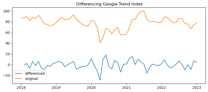
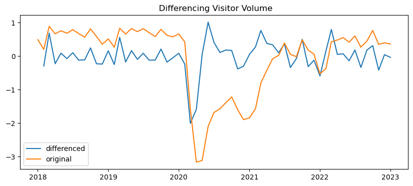
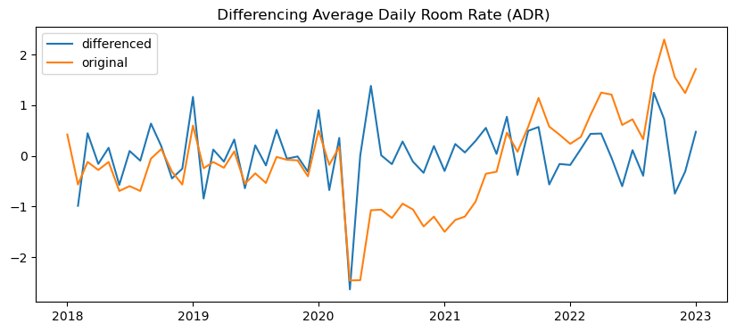
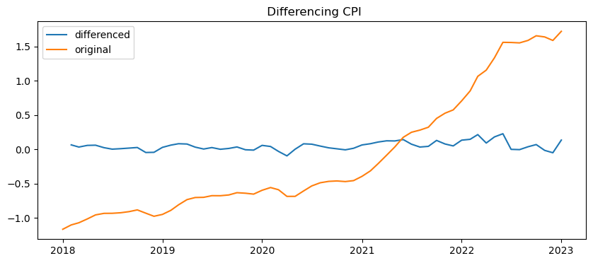
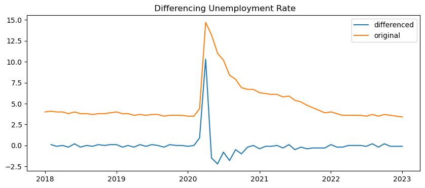
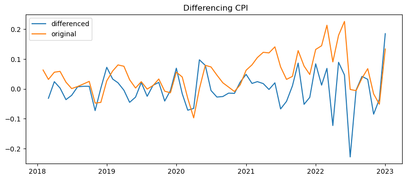
Deferencing#
Remove the trend to have only seasonal variation
If the data is non-stationary, perform a differencing technique to stationary the data
#A function to deference given series. Created a new data frame with differenced values
def defference(df):
    df_differenced = df.copy()

    for i in df.columns.values:
        df_differenced[i] = df[i].diff()
        fig, ax = plt.subplots(figsize = (10,4))
        plt.plot(df_differenced[i])
        plt.plot(df[i])
        plt.title(f' Differencing {i}')
        plt.legend(['differenced', 'original'])
        plt.show()
    return df_differenced
df_differenced  = defference(df_train)
df_differenced.head()
| Google Trend Index | Visitor Volume | Average Daily Room Rate (ADR) | CPI | Unemployment Rate | |
|---|---|---|---|---|---|
| DATE | |||||
| 2018-01-01 | NaN | NaN | NaN | NaN | NaN |
| 2018-02-01 | 0.000 | -0.293 | -0.987 | 0.063 | 0.100 |
| 2018-03-01 | 2.000 | 0.689 | 0.446 | 0.032 | -0.100 |
| 2018-04-01 | -7.000 | -0.224 | -0.159 | 0.056 | 0.000 |
| 2018-05-01 | 6.000 | 0.092 | 0.159 | 0.059 | -0.200 |
#Check stationary again
ADF_test(df_differenced.dropna())
| ADF test statistic | p-value | number of lags used | number of observations | critical values | best information criterion | Significance | |
|---|---|---|---|---|---|---|---|
| Google Trend Index | -6.838 | 0.000 | 1.000 | 58.000 | {'1%': -3.548493559596539, '5%': -2.9128365947... | 337.375 | True |
| Visitor Volume | -5.457 | 0.000 | 1.000 | 58.000 | {'1%': -3.548493559596539, '5%': -2.9128365947... | 64.918 | True |
| Average Daily Room Rate (ADR) | -9.708 | 0.000 | 0.000 | 59.000 | {'1%': -3.5463945337644063, '5%': -2.911939409... | 91.629 | True |
| CPI | -1.505 | 0.531 | 6.000 | 53.000 | {'1%': -3.560242358792829, '5%': -2.9178502070... | -144.966 | False |
| Unemployment Rate | -7.421 | 0.000 | 0.000 | 59.000 | {'1%': -3.5463945337644063, '5%': -2.911939409... | 184.413 | True |
Observation#
All time series except for CPI are stationary.
We will perform second differencing on CPI.
CPI = df_differenced.dropna().loc[:,'CPI'].to_frame()
CPI_second = defference(CPI).dropna()
ADF_test(CPI_second)
| ADF test statistic | p-value | number of lags used | number of observations | critical values | best information criterion | Significance | |
|---|---|---|---|---|---|---|---|
| CPI | -5.602 | 0.000 | 5.000 | 53.000 | {'1%': -3.560242358792829, '5%': -2.9178502070... | -140.430 | True |
#put the new CPI back
#CPI_second

all_differenced = df_differenced.copy()
all_differenced = all_differenced.iloc[2:,:]
all_differenced['CPI'] = CPI_second
all_differenced
| Google Trend Index | Visitor Volume | Average Daily Room Rate (ADR) | CPI | Unemployment Rate | |
|---|---|---|---|---|---|
| DATE | |||||
| 2018-03-01 | 2.000 | 0.689 | 0.446 | -0.032 | -0.100 |
| 2018-04-01 | -7.000 | -0.224 | -0.159 | 0.024 | 0.000 |
| 2018-05-01 | 6.000 | 0.092 | 0.159 | 0.003 | -0.200 |
| 2018-06-01 | -2.000 | -0.072 | -0.573 | -0.036 | 0.200 |
| 2018-07-01 | 6.000 | 0.105 | 0.095 | -0.022 | -0.200 |
| 2018-08-01 | -7.000 | -0.116 | -0.095 | 0.007 | 0.000 |
| 2018-09-01 | -9.000 | -0.109 | 0.637 | 0.009 | -0.100 |
| 2018-10-01 | -1.000 | 0.248 | 0.191 | 0.009 | 0.100 |
| 2018-11-01 | -3.000 | -0.225 | -0.446 | -0.073 | 0.000 |
| 2018-12-01 | 2.000 | -0.235 | -0.255 | 0.002 | 0.100 |
| 2019-01-01 | 4.000 | 0.161 | 1.163 | 0.072 | 0.100 |
| 2019-02-01 | 6.000 | -0.247 | -0.843 | 0.033 | -0.200 |
| 2019-03-01 | 4.000 | 0.564 | 0.124 | 0.020 | 0.000 |
| 2019-04-01 | -4.000 | -0.173 | -0.113 | -0.004 | -0.200 |
| 2019-05-01 | 0.000 | 0.166 | 0.322 | -0.045 | 0.100 |
| 2019-06-01 | 3.000 | -0.093 | -0.639 | -0.028 | -0.100 |
| 2019-07-01 | 6.000 | 0.087 | 0.207 | 0.021 | 0.100 |
| 2019-08-01 | -9.000 | -0.119 | -0.190 | -0.025 | 0.000 |
| 2019-09-01 | -5.000 | -0.115 | 0.514 | 0.012 | -0.200 |
| 2019-10-01 | -4.000 | 0.214 | -0.057 | 0.022 | 0.100 |
| 2019-11-01 | -3.000 | -0.176 | -0.012 | -0.041 | 0.000 |
| 2019-12-01 | 0.000 | -0.049 | -0.314 | -0.005 | 0.000 |
| 2020-01-01 | 11.000 | 0.088 | 0.901 | 0.069 | -0.100 |
| 2020-02-01 | -2.000 | -0.236 | -0.675 | -0.016 | 0.000 |
| 2020-03-01 | -11.000 | -2.005 | 0.354 | -0.071 | 0.900 |
| 2020-04-01 | -29.000 | -1.585 | -2.636 | -0.065 | 10.300 |
| 2020-05-01 | 9.000 | 0.049 | 0.006 | 0.097 | -1.500 |
| 2020-06-01 | 18.000 | 1.017 | 1.381 | 0.079 | -2.200 |
| 2020-07-01 | -3.000 | 0.415 | 0.010 | -0.006 | -0.800 |
| 2020-08-01 | -8.000 | 0.111 | -0.164 | -0.027 | -1.800 |
| 2020-09-01 | 8.000 | 0.186 | 0.283 | -0.026 | -0.500 |
| 2020-10-01 | 4.000 | 0.170 | -0.114 | -0.014 | -1.000 |
| 2020-11-01 | -14.000 | -0.381 | -0.335 | -0.015 | -0.200 |
| 2020-12-01 | 1.000 | -0.297 | 0.194 | 0.023 | 0.000 |
| 2021-01-01 | 1.000 | 0.052 | -0.299 | 0.049 | -0.400 |
| 2021-02-01 | 12.000 | 0.274 | 0.233 | 0.018 | -0.100 |
| 2021-03-01 | 15.000 | 0.768 | 0.066 | 0.024 | -0.100 |
| 2021-04-01 | 0.000 | 0.382 | 0.294 | 0.018 | 0.000 |
| 2021-05-01 | 10.000 | 0.339 | 0.552 | -0.002 | -0.300 |
| 2021-06-01 | 5.000 | 0.103 | 0.039 | 0.020 | 0.100 |
| 2021-07-01 | 1.000 | 0.369 | 0.771 | -0.067 | -0.500 |
| 2021-08-01 | -16.000 | -0.338 | -0.376 | -0.042 | -0.200 |
| 2021-09-01 | -4.000 | -0.070 | 0.493 | 0.010 | -0.400 |
| 2021-10-01 | 1.000 | 0.506 | 0.569 | 0.086 | -0.300 |
| 2021-11-01 | -1.000 | -0.309 | -0.565 | -0.052 | -0.300 |
| 2021-12-01 | -2.000 | -0.120 | -0.161 | -0.028 | -0.300 |
| 2022-01-01 | 2.000 | -0.589 | -0.180 | 0.084 | 0.100 |
| 2022-02-01 | 9.000 | 0.158 | 0.137 | 0.012 | -0.200 |
| 2022-03-01 | -1.000 | 0.799 | 0.434 | 0.069 | -0.200 |
| 2022-04-01 | -6.000 | 0.053 | 0.440 | -0.123 | 0.000 |
| 2022-05-01 | -4.000 | 0.072 | -0.039 | 0.089 | 0.000 |
| 2022-06-01 | 1.000 | -0.136 | -0.600 | 0.047 | 0.000 |
| 2022-07-01 | 7.000 | 0.186 | 0.112 | -0.228 | -0.100 |
| 2022-08-01 | 0.000 | -0.335 | -0.393 | -0.004 | 0.200 |
| 2022-09-01 | -10.000 | 0.183 | 1.244 | 0.042 | -0.200 |
| 2022-10-01 | 0.000 | 0.316 | 0.723 | 0.032 | 0.200 |
| 2022-11-01 | -9.000 | -0.416 | -0.745 | -0.085 | -0.100 |
| 2022-12-01 | 7.000 | 0.046 | -0.311 | -0.034 | -0.100 |
| 2023-01-01 | 4.000 | -0.035 | 0.475 | 0.185 | -0.100 |
8. Find optimal order (p)#
model = VAR(all_differenced)

x = model.select_order(maxlags = 8)
x.summary()
/Users/wakanamorlan/anaconda3/envs/py310/lib/python3.10/site-packages/statsmodels/tsa/base/tsa_model.py:471: ValueWarning: No frequency information was provided, so inferred frequency MS will be used.
  self._init_dates(dates, freq)
| AIC | BIC | FPE | HQIC | |
|---|---|---|---|---|
| 0 | -4.437 | -4.247* | 0.01183 | -4.365 |
| 1 | -5.076 | -3.940 | 0.006277 | -4.642* |
| 2 | -5.232 | -3.149 | 0.005530* | -4.436 |
| 3 | -5.197 | -2.167 | 0.006172 | -4.039 |
| 4 | -5.225 | -1.248 | 0.006974 | -3.705 |
| 5 | -5.467 | -0.5428 | 0.007152 | -3.585 |
| 6 | -5.549 | 0.3218 | 0.01033 | -3.306 |
| 7 | -5.838 | 0.9802 | 0.01645 | -3.233 |
| 8 | -7.250* | 0.5156 | 0.01510 | -4.282 |
x.selected_orders
{'aic': 8, 'bic': 0, 'hqic': 1, 'fpe': 2}
9. Train the model of Selected Order (p)#
model_fitted = model.fit(8)
model_fitted.summary()
Summary of Regression Results
==================================
Model: VAR
Method: OLS
Date: Mon, 22, Jul, 2024
Time: 22:51:59
--------------------------------------------------------------------
No. of Equations: 5.00000 BIC: 0.515608
Nobs: 51.0000 HQIC: -4.28227
Log likelihood: 28.0348 FPE: 0.0151044
AIC: -7.24957 Det(Omega_mle): 0.000790704
--------------------------------------------------------------------
Results for equation Google Trend Index
===================================================================================================
coefficient std. error t-stat prob
---------------------------------------------------------------------------------------------------
const 0.410035 1.406452 0.292 0.771
L1.Google Trend Index 0.005870 0.399815 0.015 0.988
L1.Visitor Volume 10.035387 4.491908 2.234 0.025
L1.Average Daily Room Rate (ADR) -9.280642 4.528390 -2.049 0.040
L1.CPI 26.066504 50.862579 0.512 0.608
L1.Unemployment Rate 2.677497 2.877610 0.930 0.352
L2.Google Trend Index -0.251914 0.401301 -0.628 0.530
L2.Visitor Volume 18.908208 14.182132 1.333 0.182
L2.Average Daily Room Rate (ADR) -10.643956 7.456218 -1.428 0.153
L2.CPI -84.112991 58.218116 -1.445 0.149
L2.Unemployment Rate -3.484508 2.777873 -1.254 0.210
L3.Google Trend Index -0.129477 0.444172 -0.292 0.771
L3.Visitor Volume -19.077949 15.466399 -1.234 0.217
L3.Average Daily Room Rate (ADR) 7.192680 9.103446 0.790 0.429
L3.CPI -49.587881 60.663208 -0.817 0.414
L3.Unemployment Rate -1.126351 3.006223 -0.375 0.708
L4.Google Trend Index 0.975413 0.647369 1.507 0.132
L4.Visitor Volume 0.876179 13.133464 0.067 0.947
L4.Average Daily Room Rate (ADR) -1.197092 7.232283 -0.166 0.869
L4.CPI -89.999304 60.807466 -1.480 0.139
L4.Unemployment Rate 1.549271 3.252287 0.476 0.634
L5.Google Trend Index -0.454882 0.562585 -0.809 0.419
L5.Visitor Volume 1.527550 13.360556 0.114 0.909
L5.Average Daily Room Rate (ADR) 8.751472 6.704038 1.305 0.192
L5.CPI -33.293876 60.974408 -0.546 0.585
L5.Unemployment Rate -3.643548 3.349614 -1.088 0.277
L6.Google Trend Index 0.476093 0.501655 0.949 0.343
L6.Visitor Volume -24.620313 17.295550 -1.424 0.155
L6.Average Daily Room Rate (ADR) 8.181529 8.948613 0.914 0.361
L6.CPI -92.608245 70.771300 -1.309 0.191
L6.Unemployment Rate -1.099318 3.389145 -0.324 0.746
L7.Google Trend Index 0.172803 0.465039 0.372 0.710
L7.Visitor Volume -1.698708 18.972209 -0.090 0.929
L7.Average Daily Room Rate (ADR) -6.492274 7.252542 -0.895 0.371
L7.CPI -35.738321 66.400841 -0.538 0.590
L7.Unemployment Rate -5.937248 3.448832 -1.722 0.085
L8.Google Trend Index 0.112063 0.442728 0.253 0.800
L8.Visitor Volume -7.894743 12.698493 -0.622 0.534
L8.Average Daily Room Rate (ADR) 7.062612 6.664380 1.060 0.289
L8.CPI -61.416610 51.746792 -1.187 0.235
L8.Unemployment Rate 0.472727 2.103812 0.225 0.822
===================================================================================================
Results for equation Visitor Volume
===================================================================================================
coefficient std. error t-stat prob
---------------------------------------------------------------------------------------------------
const 0.058927 0.092961 0.634 0.526
L1.Google Trend Index 0.020828 0.026426 0.788 0.431
L1.Visitor Volume 0.641859 0.296898 2.162 0.031
L1.Average Daily Room Rate (ADR) -0.668145 0.299309 -2.232 0.026
L1.CPI 5.851454 3.361818 1.741 0.082
L1.Unemployment Rate 0.270627 0.190199 1.423 0.155
L2.Google Trend Index -0.060233 0.026524 -2.271 0.023
L2.Visitor Volume 1.738212 0.937384 1.854 0.064
L2.Average Daily Room Rate (ADR) -0.833441 0.492827 -1.691 0.091
L2.CPI -4.691962 3.847991 -1.219 0.223
L2.Unemployment Rate -0.330188 0.183607 -1.798 0.072
L3.Google Trend Index 0.018288 0.029358 0.623 0.533
L3.Visitor Volume -1.082339 1.022269 -1.059 0.290
L3.Average Daily Room Rate (ADR) 0.119203 0.601702 0.198 0.843
L3.CPI -4.048296 4.009602 -1.010 0.313
L3.Unemployment Rate -0.058147 0.198700 -0.293 0.770
L4.Google Trend Index 0.058912 0.042789 1.377 0.169
L4.Visitor Volume -0.221610 0.868071 -0.255 0.798
L4.Average Daily Room Rate (ADR) -0.393313 0.478026 -0.823 0.411
L4.CPI -5.276802 4.019137 -1.313 0.189
L4.Unemployment Rate 0.136111 0.214964 0.633 0.527
L5.Google Trend Index -0.008843 0.037185 -0.238 0.812
L5.Visitor Volume 0.614974 0.883081 0.696 0.486
L5.Average Daily Room Rate (ADR) 0.448006 0.443111 1.011 0.312
L5.CPI -1.421932 4.030171 -0.353 0.724
L5.Unemployment Rate 0.134765 0.221396 0.609 0.543
L6.Google Trend Index 0.019500 0.033157 0.588 0.556
L6.Visitor Volume -0.089222 1.143169 -0.078 0.938
L6.Average Daily Room Rate (ADR) 0.229519 0.591468 0.388 0.698
L6.CPI -6.608550 4.677707 -1.413 0.158
L6.Unemployment Rate 0.039464 0.224009 0.176 0.860
L7.Google Trend Index 0.013121 0.030737 0.427 0.669
L7.Visitor Volume -0.388948 1.253989 -0.310 0.756
L7.Average Daily Room Rate (ADR) -0.255967 0.479365 -0.534 0.593
L7.CPI -0.571255 4.388837 -0.130 0.896
L7.Unemployment Rate -0.337262 0.227954 -1.480 0.139
L8.Google Trend Index -0.003245 0.029263 -0.111 0.912
L8.Visitor Volume -0.917526 0.839321 -1.093 0.274
L8.Average Daily Room Rate (ADR) 0.769587 0.440490 1.747 0.081
L8.CPI -6.419411 3.420261 -1.877 0.061
L8.Unemployment Rate -0.078823 0.139054 -0.567 0.571
===================================================================================================
Results for equation Average Daily Room Rate (ADR)
===================================================================================================
coefficient std. error t-stat prob
---------------------------------------------------------------------------------------------------
const 0.184358 0.109586 1.682 0.093
L1.Google Trend Index 0.011519 0.031152 0.370 0.712
L1.Visitor Volume 1.127674 0.349995 3.222 0.001
L1.Average Daily Room Rate (ADR) -1.394139 0.352838 -3.951 0.000
L1.CPI 0.786553 3.963053 0.198 0.843
L1.Unemployment Rate -0.158056 0.224214 -0.705 0.481
L2.Google Trend Index -0.014032 0.031268 -0.449 0.654
L2.Visitor Volume 0.372351 1.105027 0.337 0.736
L2.Average Daily Room Rate (ADR) -0.496255 0.580965 -0.854 0.393
L2.CPI -1.623701 4.536174 -0.358 0.720
L2.Unemployment Rate 0.103551 0.216443 0.478 0.632
L3.Google Trend Index 0.013384 0.034609 0.387 0.699
L3.Visitor Volume 0.644313 1.205093 0.535 0.593
L3.Average Daily Room Rate (ADR) -0.521198 0.709312 -0.735 0.462
L3.CPI -1.269709 4.726687 -0.269 0.788
L3.Unemployment Rate 0.195303 0.234235 0.834 0.404
L4.Google Trend Index -0.024300 0.050441 -0.482 0.630
L4.Visitor Volume 0.637095 1.023318 0.623 0.534
L4.Average Daily Room Rate (ADR) -0.223560 0.563517 -0.397 0.692
L4.CPI 2.172319 4.737928 0.458 0.647
L4.Unemployment Rate 0.211612 0.253408 0.835 0.404
L5.Google Trend Index -0.027689 0.043835 -0.632 0.528
L5.Visitor Volume 0.847673 1.041013 0.814 0.415
L5.Average Daily Room Rate (ADR) -0.328854 0.522358 -0.630 0.529
L5.CPI 3.904304 4.750935 0.822 0.411
L5.Unemployment Rate 0.319177 0.260991 1.223 0.221
L6.Google Trend Index -0.050142 0.039087 -1.283 0.200
L6.Visitor Volume 1.660452 1.347615 1.232 0.218
L6.Average Daily Room Rate (ADR) -0.712196 0.697248 -1.021 0.307
L6.CPI 3.458908 5.514278 0.627 0.530
L6.Unemployment Rate 0.358277 0.264072 1.357 0.175
L7.Google Trend Index -0.043880 0.036234 -1.211 0.226
L7.Visitor Volume 2.016214 1.478255 1.364 0.173
L7.Average Daily Room Rate (ADR) -0.747189 0.565095 -1.322 0.186
L7.CPI 3.360346 5.173746 0.649 0.516
L7.Unemployment Rate 0.085428 0.268722 0.318 0.751
L8.Google Trend Index -0.030045 0.034496 -0.871 0.384
L8.Visitor Volume 0.460586 0.989427 0.466 0.642
L8.Average Daily Room Rate (ADR) -0.042159 0.519268 -0.081 0.935
L8.CPI -1.692741 4.031948 -0.420 0.675
L8.Unemployment Rate 0.047843 0.163922 0.292 0.770
===================================================================================================
Results for equation CPI
===================================================================================================
coefficient std. error t-stat prob
---------------------------------------------------------------------------------------------------
const -0.004747 0.011359 -0.418 0.676
L1.Google Trend Index 0.005459 0.003229 1.691 0.091
L1.Visitor Volume -0.005551 0.036278 -0.153 0.878
L1.Average Daily Room Rate (ADR) -0.009415 0.036573 -0.257 0.797
L1.CPI -0.134783 0.410786 -0.328 0.743
L1.Unemployment Rate 0.017299 0.023241 0.744 0.457
L2.Google Trend Index -0.000001 0.003241 -0.000 1.000
L2.Visitor Volume 0.048284 0.114540 0.422 0.673
L2.Average Daily Room Rate (ADR) -0.003620 0.060219 -0.060 0.952
L2.CPI -0.929045 0.470192 -1.976 0.048
L2.Unemployment Rate -0.025073 0.022435 -1.118 0.264
L3.Google Trend Index 0.001270 0.003587 0.354 0.723
L3.Visitor Volume -0.169896 0.124913 -1.360 0.174
L3.Average Daily Room Rate (ADR) 0.103682 0.073523 1.410 0.158
L3.CPI -0.238559 0.489940 -0.487 0.626
L3.Unemployment Rate -0.017743 0.024279 -0.731 0.465
L4.Google Trend Index 0.008504 0.005228 1.626 0.104
L4.Visitor Volume -0.128967 0.106071 -1.216 0.224
L4.Average Daily Room Rate (ADR) 0.026489 0.058411 0.453 0.650
L4.CPI -0.475413 0.491105 -0.968 0.333
L4.Unemployment Rate 0.009198 0.026267 0.350 0.726
L5.Google Trend Index -0.002903 0.004544 -0.639 0.523
L5.Visitor Volume 0.003901 0.107905 0.036 0.971
L5.Average Daily Room Rate (ADR) 0.039590 0.054144 0.731 0.465
L5.CPI 0.113400 0.492453 0.230 0.818
L5.Unemployment Rate -0.030747 0.027053 -1.137 0.256
L6.Google Trend Index 0.002270 0.004052 0.560 0.575
L6.Visitor Volume -0.089649 0.139686 -0.642 0.521
L6.Average Daily Room Rate (ADR) 0.049465 0.072272 0.684 0.494
L6.CPI -0.789771 0.571577 -1.382 0.167
L6.Unemployment Rate 0.001619 0.027372 0.059 0.953
L7.Google Trend Index 0.002608 0.003756 0.694 0.487
L7.Visitor Volume 0.010696 0.153227 0.070 0.944
L7.Average Daily Room Rate (ADR) -0.051357 0.058574 -0.877 0.381
L7.CPI -0.097513 0.536279 -0.182 0.856
L7.Unemployment Rate -0.022189 0.027854 -0.797 0.426
L8.Google Trend Index 0.002303 0.003576 0.644 0.520
L8.Visitor Volume -0.083798 0.102558 -0.817 0.414
L8.Average Daily Room Rate (ADR) 0.071251 0.053824 1.324 0.186
L8.CPI -0.133183 0.417927 -0.319 0.750
L8.Unemployment Rate 0.019033 0.016991 1.120 0.263
===================================================================================================
Results for equation Unemployment Rate
===================================================================================================
coefficient std. error t-stat prob
---------------------------------------------------------------------------------------------------
const 0.011124 0.143801 0.077 0.938
L1.Google Trend Index 0.011450 0.040879 0.280 0.779
L1.Visitor Volume -4.113256 0.459270 -8.956 0.000
L1.Average Daily Room Rate (ADR) 1.327073 0.463000 2.866 0.004
L1.CPI -8.471917 5.200382 -1.629 0.103
L1.Unemployment Rate -0.741062 0.294218 -2.519 0.012
L2.Google Trend Index 0.083326 0.041031 2.031 0.042
L2.Visitor Volume -2.929718 1.450035 -2.020 0.043
L2.Average Daily Room Rate (ADR) 0.504587 0.762352 0.662 0.508
L2.CPI 12.533193 5.952440 2.106 0.035
L2.Unemployment Rate 0.318595 0.284020 1.122 0.262
L3.Google Trend Index 0.025215 0.045414 0.555 0.579
L3.Visitor Volume 3.090137 1.581343 1.954 0.051
L3.Average Daily Room Rate (ADR) -1.450514 0.930771 -1.558 0.119
L3.CPI 2.618104 6.202435 0.422 0.673
L3.Unemployment Rate -0.148488 0.307368 -0.483 0.629
L4.Google Trend Index -0.139344 0.066189 -2.105 0.035
L4.Visitor Volume -1.351309 1.342815 -1.006 0.314
L4.Average Daily Room Rate (ADR) 0.612487 0.739456 0.828 0.408
L4.CPI 11.104696 6.217185 1.786 0.074
L4.Unemployment Rate -0.913761 0.332526 -2.748 0.006
L5.Google Trend Index 0.143103 0.057521 2.488 0.013
L5.Visitor Volume -2.893094 1.366034 -2.118 0.034
L5.Average Daily Room Rate (ADR) -1.143588 0.685446 -1.668 0.095
L5.CPI 5.738302 6.234254 0.920 0.357
L5.Unemployment Rate 0.477645 0.342477 1.395 0.163
L6.Google Trend Index -0.096675 0.051291 -1.885 0.059
L6.Visitor Volume 3.607702 1.768362 2.040 0.041
L6.Average Daily Room Rate (ADR) -1.349623 0.914940 -1.475 0.140
L6.CPI 17.717788 7.235925 2.449 0.014
L6.Unemployment Rate -0.158711 0.346519 -0.458 0.647
L7.Google Trend Index -0.051211 0.047547 -1.077 0.281
L7.Visitor Volume 0.447582 1.939790 0.231 0.818
L7.Average Daily Room Rate (ADR) 0.077056 0.741527 0.104 0.917
L7.CPI 9.038448 6.789073 1.331 0.183
L7.Unemployment Rate 0.797560 0.352622 2.262 0.024
L8.Google Trend Index -0.046028 0.045266 -1.017 0.309
L8.Visitor Volume 3.540963 1.298342 2.727 0.006
L8.Average Daily Room Rate (ADR) -2.667656 0.681391 -3.915 0.000
L8.CPI 2.304243 5.290787 0.436 0.663
L8.Unemployment Rate -0.447450 0.215102 -2.080 0.038
===================================================================================================
Correlation matrix of residuals
Google Trend Index Visitor Volume Average Daily Room Rate (ADR) CPI Unemployment Rate
Google Trend Index 1.000000 0.441500 0.343488 0.458201 -0.576830
Visitor Volume 0.441500 1.000000 0.378825 0.466820 -0.223186
Average Daily Room Rate (ADR) 0.343488 0.378825 1.000000 0.408126 -0.499279
CPI 0.458201 0.466820 0.408126 1.000000 -0.544872
Unemployment Rate -0.576830 -0.223186 -0.499279 -0.544872 1.000000
10. Check for serial Correlation of Residuals using Durbin Watson Statistic#
from statsmodels.stats.stattools import durbin_watson
out = durbin_watson(model_fitted.resid)  #Residuals of response variable resulting from estimated coefficients
out
array([1.7555842 , 1.53950947, 1.71539114, 1.72416996, 1.91597751])
for col, val in zip(all_differenced.columns, out):
    print(col, ":", round(val,2))
Google Trend Index : 1.76
Visitor Volume : 1.54
Average Daily Room Rate (ADR) : 1.72
CPI : 1.72
Unemployment Rate : 1.92
11. Forecast#
#get the lag order
lag_order = model_fitted.k_ar
print(f'lag order: {lag_order}')


#input data for forecasting
forecast_input = all_differenced.values[-lag_order:]
forecast_input
lag order: 8
array([[ 1.00000000e+00, -1.35871562e-01, -5.99709162e-01,
         4.65717349e-02,  0.00000000e+00],
       [ 7.00000000e+00,  1.85613239e-01,  1.11729255e-01,
        -2.27796529e-01, -1.00000000e-01],
       [ 0.00000000e+00, -3.34949551e-01, -3.92803135e-01,
        -3.93722397e-03,  2.00000000e-01],
       [-1.00000000e+01,  1.83165103e-01,  1.24430102e+00,
         4.17345740e-02, -2.00000000e-01],
       [ 0.00000000e+00,  3.16032134e-01,  7.22897827e-01,
         3.18915141e-02,  2.00000000e-01],
       [-9.00000000e+00, -4.15849326e-01, -7.45180015e-01,
        -8.46503153e-02, -1.00000000e-01],
       [ 7.00000000e+00,  4.64033099e-02, -3.10995675e-01,
        -3.44788327e-02, -1.00000000e-01],
       [ 4.00000000e+00, -3.54979757e-02,  4.74610595e-01,
         1.84880788e-01, -1.00000000e-01]])
#Forecast
fc = model_fitted.forecast(y=forecast_input, steps=nobs)
df_forecast = pd.DataFrame(fc, index=df.index[-nobs:], columns = df.columns + '_fc')
df_forecast
| Google Trend Index_fc | Visitor Volume_fc | Average Daily Room Rate (ADR)_fc | CPI_fc | Unemployment Rate_fc | |
|---|---|---|---|---|---|
| DATE | |||||
| 2023-02-01 | 34.025 | 1.182 | -0.985 | 0.101 | -6.529 |
| 2023-03-01 | 0.229 | 1.767 | 4.086 | -0.074 | 1.145 |
| 2023-04-01 | 9.459 | 0.040 | -4.932 | 0.075 | -4.110 |
| 2023-05-01 | -15.978 | 1.077 | 7.487 | -0.070 | -0.255 |
12. Revert the differenced values#
def de_defference(col_name, df_train, df_forecast, second_diff=False):
    """
    A function to revert back to difference values to the original scale.
    """
    df_fc = df_forecast.copy()
    if second_diff == True:
        df_fc[col_name+'_fc']=(df_train[loc_name].iloc[-1]-df_train[col_name].iloc[-2])+df_fc[col_name+'_fc'].cumsum()

    df_fc[col_name+"_forecast"] = df_train[col_name].iloc[-1]+df_fc[col_name+'_fc'].cumsum()

    return df_fc[col_name+"_forecast"].to_frame()
df_result = de_defference('Google Trend Index', df_train,df_forecast)
df_result
| Google Trend Index_forecast | |
|---|---|
| DATE | |
| 2023-02-01 | 112.025 |
| 2023-03-01 | 112.254 |
| 2023-04-01 | 121.713 |
| 2023-05-01 | 105.735 |
fig, axes = plt.subplots()

df_result['Google Trend Index_forecast'].plot(legend=True)
df_test['Google Trend Index'][-nobs:].plot(legend=True)
axes.set_title("Forecaset vs Actual")

;
''
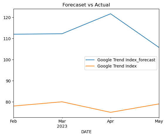
12. Evaluate the model#
Root Mean Squared Error (RMSE)
Mean Absolute Error(MAE)
Mean Squiared Error (MSE)
Mean Absolute Percentage Error (MAPE)
from statsmodels.tools.eval_measures import rmse, meanabs, mse
from sklearn.metrics import mean_absolute_percentage_error as mape
measures = [rmse, meanabs, mse, mape]
#Create a function to show the dataframe of the result for a given model
def eval_summary(model_name, df_result, df_test):
    fc_google_trend = df_result['Google Trend Index_forecast']
    actual_google_trend = df_test['Google Trend Index'][-nobs:]
    evaluations = {'RMSE':[], 'MAE':[],'MSE':[],'MAPE':[]}

    for m, e in zip(measures, evaluations):
        measure = m(fc_google_trend, actual_google_trend)
        evaluations[e].append(measure)

    evaluations.update({'Model_name':[]})
    evaluations['Model_name'] = model_name

    summary = pd.DataFrame.from_dict(evaluations)
    return summary
eval_summary('Model_1', df_result, df_test)
| RMSE | MAE | MSE | MAPE | Model_name | |
|---|---|---|---|---|---|
| 0 | 35.689 | 34.932 | 1273.714 | 0.307 | Model_1 |
13. Find the best combination of input variables#
#create possible combinations of input variables

from itertools import combinations
input_vars = list(df.columns.values)
input_vars.remove('Google Trend Index')

combos = []
for n in range(1, len(input_vars)+1):
    combos+=list(combinations(input_vars,n))

variables_combos = []
for i in combos:
    variables_combos.append(list(i))

print(variables_combos)

len(variables_combos)
[['Visitor Volume'], ['Average Daily Room Rate (ADR)'], ['CPI'], ['Unemployment Rate'], ['Visitor Volume', 'Average Daily Room Rate (ADR)'], ['Visitor Volume', 'CPI'], ['Visitor Volume', 'Unemployment Rate'], ['Average Daily Room Rate (ADR)', 'CPI'], ['Average Daily Room Rate (ADR)', 'Unemployment Rate'], ['CPI', 'Unemployment Rate'], ['Visitor Volume', 'Average Daily Room Rate (ADR)', 'CPI'], ['Visitor Volume', 'Average Daily Room Rate (ADR)', 'Unemployment Rate'], ['Visitor Volume', 'CPI', 'Unemployment Rate'], ['Average Daily Room Rate (ADR)', 'CPI', 'Unemployment Rate'], ['Visitor Volume', 'Average Daily Room Rate (ADR)', 'CPI', 'Unemployment Rate']]
15
Repeat the process from 8#
list(range(1,len(variables_combos)+1))

model_names = []
for i in list(range(1,len(variables_combos)+1)):
    model_names.append("model_"+str(i))

model_names
['model_1',
 'model_2',
 'model_3',
 'model_4',
 'model_5',
 'model_6',
 'model_7',
 'model_8',
 'model_9',
 'model_10',
 'model_11',
 'model_12',
 'model_13',
 'model_14',
 'model_15']
tuples = [(key, value)
          for i, (key, value) in enumerate(zip(model_names, variables_combos))]
all_models = dict(tuples)
all_models
{'model_1': ['Visitor Volume'],
 'model_2': ['Average Daily Room Rate (ADR)'],
 'model_3': ['CPI'],
 'model_4': ['Unemployment Rate'],
 'model_5': ['Visitor Volume', 'Average Daily Room Rate (ADR)'],
 'model_6': ['Visitor Volume', 'CPI'],
 'model_7': ['Visitor Volume', 'Unemployment Rate'],
 'model_8': ['Average Daily Room Rate (ADR)', 'CPI'],
 'model_9': ['Average Daily Room Rate (ADR)', 'Unemployment Rate'],
 'model_10': ['CPI', 'Unemployment Rate'],
 'model_11': ['Visitor Volume', 'Average Daily Room Rate (ADR)', 'CPI'],
 'model_12': ['Visitor Volume',
  'Average Daily Room Rate (ADR)',
  'Unemployment Rate'],
 'model_13': ['Visitor Volume', 'CPI', 'Unemployment Rate'],
 'model_14': ['Average Daily Room Rate (ADR)', 'CPI', 'Unemployment Rate'],
 'model_15': ['Visitor Volume',
  'Average Daily Room Rate (ADR)',
  'CPI',
  'Unemployment Rate']}
#Function to find try all possible combos
def build_VAR(model_name,differenced_df=all_differenced):
## Create a subset of dataframe with a given input variable combination ##
a = all_models.get(model_name)
a.insert(0,'Google Trend Index')
b = a.copy()
print(b)
subset_df = differenced_df[b]
## create a new VAR model with the selected variables ##
model = VAR(subset_df)
## Find the optimal order (p) for a given VAR model ##
x = model.select_order(maxlags = 7)
print(x.summary())
selected_p = x.selected_orders['aic']
## Train the model with the selected order(p) ##
if selected_p >0:
model_fitted = model.fit(selected_p)
else: model_fitted = model.fit(None)
print(model_fitted.summary())
## Check for serial correlation of residuals using Durbin Watson Statistics ##
from statsmodels.stats.stattools import durbin_watson
out = durbin_watson(model_fitted.resid) #Residuals of response variable resulting from estimated coefficients
print ("\n\n/// The Durbin Watson Test ///")
for col, val in zip(subset_df.columns, out):
print(col, ":", round(val,2))
## Forecast ##
lag_order = model_fitted.k_ar
#input data for forecasting
forecast_input = subset_df.values[-lag_order:]
fc = model_fitted.forecast(y=forecast_input, steps=nobs)
df_forecast = pd.DataFrame(fc, index=df.index[-nobs:], columns = subset_df.columns + '_fc')
df_forecast
## Inverse the differenced values ##
df_result = de_defference('Google Trend Index', df_train,df_forecast)
df_result
## Plot the result ##
fig, axes = plt.subplots()
df_result['Google Trend Index_forecast'].plot(legend=True)
df_test['Google Trend Index'][-nobs:].plot(legend=True)
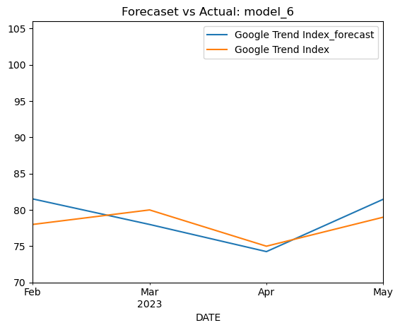
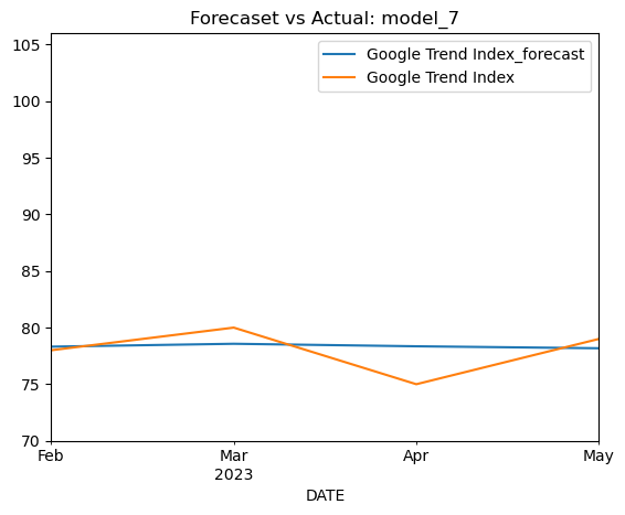
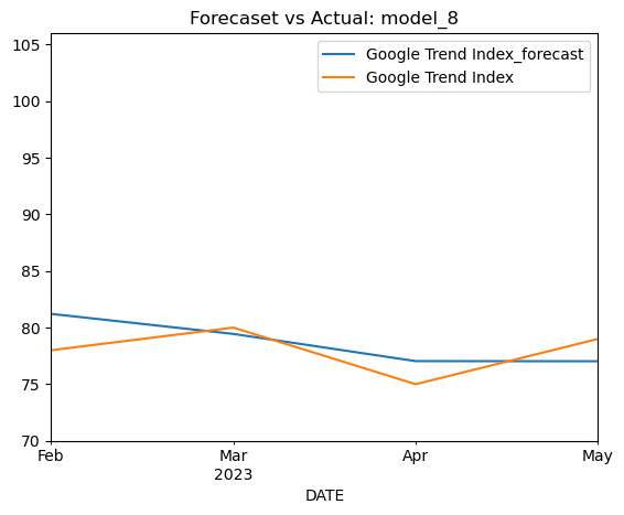
axes.set_title(f"Forecaset vs Actual: {model_name}")
axes.set_ylim(70, 106)
## Evaluate the model
summary = eval_summary(model_name, df_result, df_test)
return summary
model_1 = build_VAR("model_1")
model_1
['Google Trend Index', 'Visitor Volume']
 VAR Order Selection (* highlights the minimums)
=================================================
      AIC         BIC         FPE         HQIC
-------------------------------------------------
0       2.261      2.336*       9.596      2.290*
1       2.270       2.495       9.685       2.357
2      2.238*       2.613      9.386*       2.382
3       2.283       2.808       9.837       2.484
4       2.398       3.073       11.07       2.657
5       2.356       3.182       10.69       2.673
6       2.438       3.414       11.70       2.812
7       2.469       3.594       12.21       2.900
-------------------------------------------------
  Summary of Regression Results
==================================
Model:                         VAR
Method:                        OLS
Date:           Mon, 22, Jul, 2024
Time:                     22:52:00
--------------------------------------------------------------------
No. of Equations:         2.00000    BIC:                    2.49470
Nobs:                     57.0000    HQIC:                   2.27557
Log likelihood:          -212.643    FPE:                    8.47548
AIC:                      2.13627    Det(Omega_mle):         7.16359
--------------------------------------------------------------------
Results for equation Google Trend Index
========================================================================================
                           coefficient       std. error           t-stat            prob
----------------------------------------------------------------------------------------
const                        -0.128336         1.011580           -0.127           0.899
L1.Google Trend Index         0.025674         0.165578            0.155           0.877
L1.Visitor Volume             3.727946         2.997797            1.244           0.214
L2.Google Trend Index        -0.291790         0.165351           -1.765           0.078
L2.Visitor Volume            -1.994707         2.837904           -0.703           0.482
========================================================================================

Results for equation Visitor Volume
========================================================================================
                           coefficient       std. error           t-stat            prob
----------------------------------------------------------------------------------------
const                        -0.005717         0.057143           -0.100           0.920
L1.Google Trend Index         0.003099         0.009353            0.331           0.740
L1.Visitor Volume             0.390197         0.169341            2.304           0.021
L2.Google Trend Index        -0.013666         0.009340           -1.463           0.143
L2.Visitor Volume            -0.081612         0.160309           -0.509           0.611
========================================================================================

Correlation matrix of residuals
                      Google Trend Index  Visitor Volume
Google Trend Index              1.000000        0.577775
Visitor Volume                  0.577775        1.000000


/// The Durbin Watson Test ///
Google Trend Index : 1.99
Visitor Volume : 1.97
/Users/wakanamorlan/anaconda3/envs/py310/lib/python3.10/site-packages/statsmodels/tsa/base/tsa_model.py:471: ValueWarning: No frequency information was provided, so inferred frequency MS will be used.
  self._init_dates(dates, freq)
| RMSE | MAE | MSE | MAPE | Model_name | |
|---|---|---|---|---|---|
| 0 | 3.821 | 3.263 | 14.597 | 0.044 | model_1 |
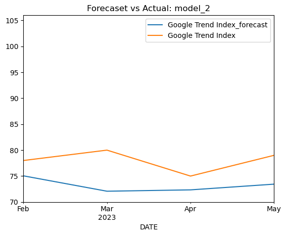
model_2= build_VAR('model_2')
model_2
['Google Trend Index', 'Average Daily Room Rate (ADR)']
 VAR Order Selection (* highlights the minimums)
=================================================
      AIC         BIC         FPE         HQIC
-------------------------------------------------
0       3.009      3.084*       20.27      3.038*
1       2.992       3.217       19.92       3.078
2      2.911*       3.286      18.40*       3.055
3       2.998       3.523       20.11       3.199
4       3.140       3.815       23.26       3.399
5       3.230       4.055       25.60       3.546
6       3.324       4.300       28.39       3.698
7       3.319       4.445       28.58       3.751
-------------------------------------------------
  Summary of Regression Results
==================================
Model:                         VAR
Method:                        OLS
Date:           Mon, 22, Jul, 2024
Time:                     22:52:00
--------------------------------------------------------------------
No. of Equations:         2.00000    BIC:                    3.21692
Nobs:                     57.0000    HQIC:                   2.99779
Log likelihood:          -233.226    FPE:                    17.4510
AIC:                      2.85849    Det(Omega_mle):         14.7498
--------------------------------------------------------------------
Results for equation Google Trend Index
===================================================================================================
                                      coefficient       std. error           t-stat            prob
---------------------------------------------------------------------------------------------------
const                                    0.068124         0.956870            0.071           0.943
L1.Google Trend Index                    0.312272         0.140530            2.222           0.026
L1.Average Daily Room Rate (ADR)        -5.262479         1.784561           -2.949           0.003
L2.Google Trend Index                   -0.293906         0.141848           -2.072           0.038
L2.Average Daily Room Rate (ADR)        -0.908529         1.919397           -0.473           0.636
===================================================================================================

Results for equation Average Daily Room Rate (ADR)
===================================================================================================
                                      coefficient       std. error           t-stat            prob
---------------------------------------------------------------------------------------------------
const                                    0.057845         0.079357            0.729           0.466
L1.Google Trend Index                    0.008504         0.011655            0.730           0.466
L1.Average Daily Room Rate (ADR)        -0.321878         0.148001           -2.175           0.030
L2.Google Trend Index                    0.011764         0.011764            1.000           0.317
L2.Average Daily Room Rate (ADR)        -0.237902         0.159183           -1.495           0.135
===================================================================================================

Correlation matrix of residuals
                                 Google Trend Index  Average Daily Room Rate (ADR)
Google Trend Index                         1.000000                       0.433051
Average Daily Room Rate (ADR)              0.433051                       1.000000


/// The Durbin Watson Test ///
Google Trend Index : 1.98
Average Daily Room Rate (ADR) : 2.1
/Users/wakanamorlan/anaconda3/envs/py310/lib/python3.10/site-packages/statsmodels/tsa/base/tsa_model.py:471: ValueWarning: No frequency information was provided, so inferred frequency MS will be used.
  self._init_dates(dates, freq)
| RMSE | MAE | MSE | MAPE | Model_name | |
|---|---|---|---|---|---|
| 0 | 5.230 | 4.772 | 27.349 | 0.065 | model_2 |
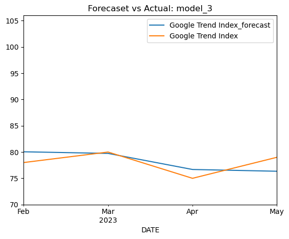
model_3 = build_VAR('model_3')
model_3
['Google Trend Index', 'CPI']
 VAR Order Selection (* highlights the minimums)
=================================================
      AIC         BIC         FPE         HQIC
-------------------------------------------------
0      -1.404     -1.329*      0.2456      -1.375
1      -1.344      -1.118      0.2610      -1.257
2     -1.608*      -1.233     0.2005*     -1.464*
3      -1.477     -0.9521      0.2290      -1.276
4      -1.604     -0.9286      0.2025      -1.345
5      -1.532     -0.7065      0.2189      -1.216
6      -1.604     -0.6289      0.2054      -1.230
7      -1.490     -0.3641      0.2331      -1.058
-------------------------------------------------
  Summary of Regression Results
==================================
Model:                         VAR
Method:                        OLS
Date:           Mon, 22, Jul, 2024
Time:                     22:52:00
--------------------------------------------------------------------
No. of Equations:         2.00000    BIC:                   -1.35193
Nobs:                     57.0000    HQIC:                  -1.57106
Log likelihood:          -103.014    FPE:                   0.180964
AIC:                     -1.71036    Det(Omega_mle):        0.152953
--------------------------------------------------------------------
Results for equation Google Trend Index
========================================================================================
                           coefficient       std. error           t-stat            prob
----------------------------------------------------------------------------------------
const                        -0.112317         1.012878           -0.111           0.912
L1.Google Trend Index         0.092535         0.138890            0.666           0.505
L1.CPI                       23.358539        19.405394            1.204           0.229
L2.Google Trend Index        -0.320017         0.135615           -2.360           0.018
L2.CPI                        8.355535        19.752737            0.423           0.672
========================================================================================

Results for equation CPI
========================================================================================
                           coefficient       std. error           t-stat            prob
----------------------------------------------------------------------------------------
const                         0.000191         0.007192            0.027           0.979
L1.Google Trend Index         0.001163         0.000986            1.179           0.238
L1.CPI                       -0.216112         0.137795           -1.568           0.117
L2.Google Trend Index        -0.001362         0.000963           -1.414           0.157
L2.CPI                       -0.487002         0.140261           -3.472           0.001
========================================================================================

Correlation matrix of residuals
                      Google Trend Index       CPI
Google Trend Index              1.000000  0.326887
CPI                             0.326887  1.000000


/// The Durbin Watson Test ///
Google Trend Index : 2.02
CPI : 1.95
/Users/wakanamorlan/anaconda3/envs/py310/lib/python3.10/site-packages/statsmodels/tsa/base/tsa_model.py:471: ValueWarning: No frequency information was provided, so inferred frequency MS will be used.
  self._init_dates(dates, freq)
| RMSE | MAE | MSE | MAPE | Model_name | |
|---|---|---|---|---|---|
| 0 | 1.880 | 1.661 | 3.535 | 0.021 | model_3 |
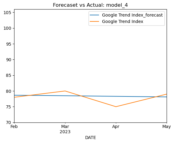
model_4 = build_VAR('model_4')
model_4
['Google Trend Index', 'Unemployment Rate']
 VAR Order Selection (* highlights the minimums)
=================================================
      AIC         BIC         FPE         HQIC
-------------------------------------------------
0      4.708*      4.783*      110.9*      4.737*
1       4.796       5.021       121.1       4.882
2       4.779       5.154       119.2       4.923
3       4.890       5.415       133.3       5.091
4       4.938       5.614       140.5       5.197
5       4.999       5.824       150.2       5.315
6       5.054       6.030       160.1       5.428
7       4.966       6.091       148.3       5.397
-------------------------------------------------
  Summary of Regression Results
==================================
Model:                         VAR
Method:                        OLS
Date:           Mon, 22, Jul, 2024
Time:                     22:52:00
--------------------------------------------------------------------
No. of Equations:         2.00000    BIC:                    4.87980
Nobs:                     58.0000    HQIC:                   4.74967
Log likelihood:          -293.930    FPE:                    106.360
AIC:                      4.66665    Det(Omega_mle):         96.1560
--------------------------------------------------------------------
Results for equation Google Trend Index
========================================================================================
                           coefficient       std. error           t-stat            prob
----------------------------------------------------------------------------------------
const                        -0.128968         1.037890           -0.124           0.901
L1.Google Trend Index         0.221221         0.156971            1.409           0.159
L1.Unemployment Rate          1.073310         0.852862            1.258           0.208
========================================================================================

Results for equation Unemployment Rate
========================================================================================
                           coefficient       std. error           t-stat            prob
----------------------------------------------------------------------------------------
const                        -0.019772         0.191731           -0.103           0.918
L1.Google Trend Index        -0.037765         0.028997           -1.302           0.193
L1.Unemployment Rate         -0.093084         0.157550           -0.591           0.555
========================================================================================

Correlation matrix of residuals
                      Google Trend Index  Unemployment Rate
Google Trend Index              1.000000          -0.525313
Unemployment Rate              -0.525313           1.000000


/// The Durbin Watson Test ///
Google Trend Index : 1.96
Unemployment Rate : 2.0
/Users/wakanamorlan/anaconda3/envs/py310/lib/python3.10/site-packages/statsmodels/tsa/base/tsa_model.py:471: ValueWarning: No frequency information was provided, so inferred frequency MS will be used.
  self._init_dates(dates, freq)
| RMSE | MAE | MSE | MAPE | Model_name | |
|---|---|---|---|---|---|
| 0 | 1.894 | 1.586 | 3.586 | 0.020 | model_4 |
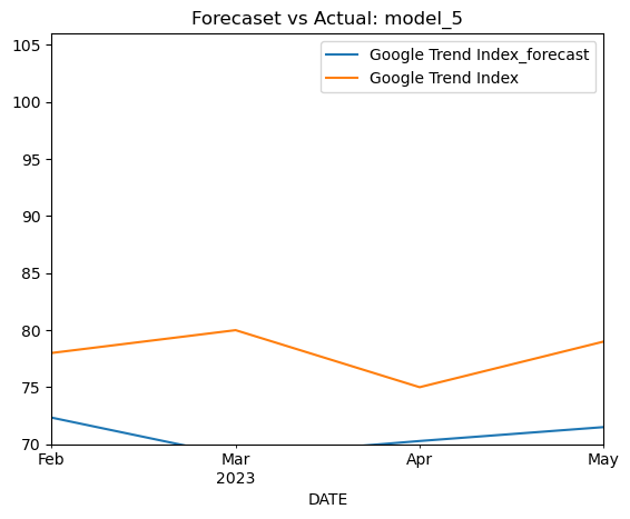
model_5 = build_VAR('model_5')
model_5
['Google Trend Index', 'Visitor Volume', 'Average Daily Room Rate (ADR)']
 VAR Order Selection (* highlights the minimums)
=================================================
      AIC         BIC         FPE         HQIC
-------------------------------------------------
0      0.9124      1.025*       2.490      0.9555
1      0.7233       1.174       2.063     0.8959*
2     0.6295*       1.417      1.886*      0.9316
3      0.7363       1.862       2.119       1.168
4      0.9245       2.388       2.604       1.486
5       1.060       2.861       3.070       1.750
6       1.170       3.309       3.583       1.990
7       1.198       3.674       3.926       2.147
-------------------------------------------------
  Summary of Regression Results
==================================
Model:                         VAR
Method:                        OLS
Date:           Mon, 22, Jul, 2024
Time:                     22:52:00
--------------------------------------------------------------------
No. of Equations:         3.00000    BIC:                    1.22196
Nobs:                     57.0000    HQIC:                  0.761782
Log likelihood:          -235.012    FPE:                    1.60479
AIC:                     0.469256    Det(Omega_mle):         1.13371
--------------------------------------------------------------------
Results for equation Google Trend Index
===================================================================================================
                                      coefficient       std. error           t-stat            prob
---------------------------------------------------------------------------------------------------
const                                    0.187958         0.891368            0.211           0.833
L1.Google Trend Index                    0.050736         0.155594            0.326           0.744
L1.Visitor Volume                        8.874502         2.900685            3.059           0.002
L1.Average Daily Room Rate (ADR)        -8.398308         1.988138           -4.224           0.000
L2.Google Trend Index                   -0.406602         0.150465           -2.702           0.007
L2.Visitor Volume                        2.426412         2.926933            0.829           0.407
L2.Average Daily Room Rate (ADR)        -3.147999         2.113996           -1.489           0.136
===================================================================================================

Results for equation Visitor Volume
===================================================================================================
                                      coefficient       std. error           t-stat            prob
---------------------------------------------------------------------------------------------------
const                                    0.006013         0.056250            0.107           0.915
L1.Google Trend Index                    0.002080         0.009819            0.212           0.832
L1.Visitor Volume                        0.552545         0.183049            3.019           0.003
L1.Average Daily Room Rate (ADR)        -0.254065         0.125462           -2.025           0.043
L2.Google Trend Index                   -0.016172         0.009495           -1.703           0.089
L2.Visitor Volume                        0.088352         0.184705            0.478           0.632
L2.Average Daily Room Rate (ADR)        -0.157926         0.133405           -1.184           0.236
===================================================================================================

Results for equation Average Daily Room Rate (ADR)
===================================================================================================
                                      coefficient       std. error           t-stat            prob
---------------------------------------------------------------------------------------------------
const                                    0.070114         0.068516            1.023           0.306
L1.Google Trend Index                   -0.020332         0.011960           -1.700           0.089
L1.Visitor Volume                        0.986556         0.222963            4.425           0.000
L1.Average Daily Room Rate (ADR)        -0.636296         0.152820           -4.164           0.000
L2.Google Trend Index                    0.002622         0.011566            0.227           0.821
L2.Visitor Volume                        0.128031         0.224981            0.569           0.569
L2.Average Daily Room Rate (ADR)        -0.436685         0.162494           -2.687           0.007
===================================================================================================

Correlation matrix of residuals
                                 Google Trend Index  Visitor Volume  Average Daily Room Rate (ADR)
Google Trend Index                         1.000000        0.530464                       0.281006
Visitor Volume                             0.530464        1.000000                       0.487946
Average Daily Room Rate (ADR)              0.281006        0.487946                       1.000000


/// The Durbin Watson Test ///
Google Trend Index : 2.0
Visitor Volume : 1.97
Average Daily Room Rate (ADR) : 2.25
/Users/wakanamorlan/anaconda3/envs/py310/lib/python3.10/site-packages/statsmodels/tsa/base/tsa_model.py:471: ValueWarning: No frequency information was provided, so inferred frequency MS will be used.
  self._init_dates(dates, freq)
| RMSE | MAE | MSE | MAPE | Model_name | |
|---|---|---|---|---|---|
| 0 | 7.623 | 7.229 | 58.103 | 0.103 | model_5 |
model_6 = build_VAR('model_6')
model_6
['Google Trend Index', 'Visitor Volume', 'CPI']
 VAR Order Selection (* highlights the minimums)
=================================================
      AIC         BIC         FPE         HQIC
-------------------------------------------------
0      -3.356     -3.243*     0.03489     -3.312*
1      -3.303      -2.853     0.03681      -3.130
2      -3.457      -2.669     0.03167      -3.155
3      -3.286      -2.160     0.03794      -2.855
4      -3.594      -2.131    0.02839*      -3.033
5      -3.498      -1.696     0.03220      -2.807
6     -3.644*      -1.505     0.02909      -2.824
7      -3.400     -0.9231     0.03957      -2.450
-------------------------------------------------
  Summary of Regression Results
==================================
Model:                         VAR
Method:                        OLS
Date:           Mon, 22, Jul, 2024
Time:                     22:52:01
--------------------------------------------------------------------
No. of Equations:         3.00000    BIC:                   -1.57353
Nobs:                     53.0000    HQIC:                  -2.87766
Log likelihood:          -70.7594    FPE:                  0.0275280
AIC:                     -3.69252    Det(Omega_mle):       0.0109801
--------------------------------------------------------------------
Results for equation Google Trend Index
========================================================================================
                           coefficient       std. error           t-stat            prob
----------------------------------------------------------------------------------------
const                        -0.261741         1.076633           -0.243           0.808
L1.Google Trend Index        -0.097321         0.231259           -0.421           0.674
L1.Visitor Volume             5.926401         3.815709            1.553           0.120
L1.CPI                       14.839599        31.084849            0.477           0.633
L2.Google Trend Index        -0.363349         0.227952           -1.594           0.111
L2.Visitor Volume            -3.604941         3.751384           -0.961           0.337
L2.CPI                       34.899393        30.676124            1.138           0.255
L3.Google Trend Index        -0.187748         0.206698           -0.908           0.364
L3.Visitor Volume            -0.889300         3.863143           -0.230           0.818
L3.CPI                       22.947340        33.204686            0.691           0.490
L4.Google Trend Index        -0.249739         0.214814           -1.163           0.245
L4.Visitor Volume             4.417707         3.741812            1.181           0.238
L4.CPI                       58.033396        34.139706            1.700           0.089
L5.Google Trend Index        -0.151172         0.210402           -0.718           0.472
L5.Visitor Volume             0.532614         4.737704            0.112           0.910
L5.CPI                       -0.547545        29.466808           -0.019           0.985
L6.Google Trend Index        -0.052968         0.230153           -0.230           0.818
L6.Visitor Volume            -1.761387         4.390918           -0.401           0.688
L6.CPI                       -2.454041        28.459655           -0.086           0.931
========================================================================================

Results for equation Visitor Volume
========================================================================================
                           coefficient       std. error           t-stat            prob
----------------------------------------------------------------------------------------
const                        -0.002531         0.063740           -0.040           0.968
L1.Google Trend Index         0.007375         0.013691            0.539           0.590
L1.Visitor Volume             0.422507         0.225903            1.870           0.061
L1.CPI                        0.284373         1.840333            0.155           0.877
L2.Google Trend Index        -0.014923         0.013496           -1.106           0.269
L2.Visitor Volume            -0.085666         0.222095           -0.386           0.700
L2.CPI                       -0.625100         1.816135           -0.344           0.731
L3.Google Trend Index         0.015238         0.012237            1.245           0.213
L3.Visitor Volume            -0.196524         0.228712           -0.859           0.390
L3.CPI                       -1.103097         1.965834           -0.561           0.575
L4.Google Trend Index         0.000682         0.012718            0.054           0.957
L4.Visitor Volume            -0.208482         0.221528           -0.941           0.347
L4.CPI                        2.363502         2.021191            1.169           0.242
L5.Google Trend Index         0.012882         0.012457            1.034           0.301
L5.Visitor Volume            -0.044258         0.280489           -0.158           0.875
L5.CPI                       -1.090550         1.744539           -0.625           0.532
L6.Google Trend Index        -0.002498         0.013626           -0.183           0.855
L6.Visitor Volume            -0.031376         0.259958           -0.121           0.904
L6.CPI                        0.293703         1.684912            0.174           0.862
========================================================================================

Results for equation CPI
========================================================================================
                           coefficient       std. error           t-stat            prob
----------------------------------------------------------------------------------------
const                         0.001021         0.006239            0.164           0.870
L1.Google Trend Index         0.001382         0.001340            1.031           0.302
L1.Visitor Volume             0.005027         0.022112            0.227           0.820
L1.CPI                       -0.198552         0.180133           -1.102           0.270
L2.Google Trend Index        -0.001367         0.001321           -1.035           0.301
L2.Visitor Volume            -0.021910         0.021739           -1.008           0.314
L2.CPI                       -0.446637         0.177764           -2.513           0.012
L3.Google Trend Index         0.000512         0.001198            0.427           0.669
L3.Visitor Volume             0.020303         0.022386            0.907           0.364
L3.CPI                       -0.029325         0.192417           -0.152           0.879
L4.Google Trend Index        -0.000066         0.001245           -0.053           0.958
L4.Visitor Volume            -0.065312         0.021683           -3.012           0.003
L4.CPI                        0.068704         0.197835            0.347           0.728
L5.Google Trend Index        -0.000609         0.001219           -0.500           0.617
L5.Visitor Volume             0.020791         0.027454            0.757           0.449
L5.CPI                        0.121378         0.170757            0.711           0.477
L6.Google Trend Index        -0.001389         0.001334           -1.041           0.298
L6.Visitor Volume             0.042271         0.025445            1.661           0.097
L6.CPI                       -0.421098         0.164920           -2.553           0.011
========================================================================================

Correlation matrix of residuals
                      Google Trend Index  Visitor Volume       CPI
Google Trend Index              1.000000        0.633126  0.524471
Visitor Volume                  0.633126        1.000000  0.458120
CPI                             0.524471        0.458120  1.000000


/// The Durbin Watson Test ///
Google Trend Index : 1.96
Visitor Volume : 1.94
CPI : 1.99
/Users/wakanamorlan/anaconda3/envs/py310/lib/python3.10/site-packages/statsmodels/tsa/base/tsa_model.py:471: ValueWarning: No frequency information was provided, so inferred frequency MS will be used.
  self._init_dates(dates, freq)
| RMSE | MAE | MSE | MAPE | Model_name | |
|---|---|---|---|---|---|
| 0 | 2.401 | 2.184 | 5.763 | 0.027 | model_6 |
model_7 = build_VAR('model_7')
model_7
['Google Trend Index', 'Visitor Volume', 'Unemployment Rate']
 VAR Order Selection (* highlights the minimums)
=================================================
      AIC         BIC         FPE         HQIC
-------------------------------------------------
0       2.649       2.762       14.15       2.693
1      2.232*      2.682*      9.323*      2.404*
2       2.337       3.125       10.40       2.639
3       2.447       3.572       11.72       2.878
4       2.653       4.117       14.67       3.214
5       2.505       4.306       13.03       3.196
6       2.595       4.733       14.89       3.415
7       2.381       4.857       12.82       3.330
-------------------------------------------------
  Summary of Regression Results
==================================
Model:                         VAR
Method:                        OLS
Date:           Mon, 22, Jul, 2024
Time:                     22:52:01
--------------------------------------------------------------------
No. of Equations:         3.00000    BIC:                    2.43245
Nobs:                     58.0000    HQIC:                   2.17221
Log likelihood:          -293.074    FPE:                    7.43956
AIC:                      2.00615    Det(Omega_mle):         6.09055
--------------------------------------------------------------------
Results for equation Google Trend Index
========================================================================================
                           coefficient       std. error           t-stat            prob
----------------------------------------------------------------------------------------
const                        -0.146161         1.043347           -0.140           0.889
L1.Google Trend Index         0.166067         0.177541            0.935           0.350
L1.Visitor Volume             2.062959         3.046975            0.677           0.498
L1.Unemployment Rate          1.282753         0.911209            1.408           0.159
========================================================================================

Results for equation Visitor Volume
========================================================================================
                           coefficient       std. error           t-stat            prob
----------------------------------------------------------------------------------------
const                        -0.007585         0.058084           -0.131           0.896
L1.Google Trend Index         0.009051         0.009884            0.916           0.360
L1.Visitor Volume             0.300876         0.169629            1.774           0.076
L1.Unemployment Rate          0.049222         0.050728            0.970           0.332
========================================================================================

Results for equation Unemployment Rate
========================================================================================
                           coefficient       std. error           t-stat            prob
----------------------------------------------------------------------------------------
const                         0.001630         0.152134            0.011           0.991
L1.Google Trend Index         0.030891         0.025888            1.193           0.233
L1.Visitor Volume            -2.567981         0.444288           -5.780           0.000
L1.Unemployment Rate         -0.353801         0.132866           -2.663           0.008
========================================================================================

Correlation matrix of residuals
                      Google Trend Index  Visitor Volume  Unemployment Rate
Google Trend Index              1.000000        0.619260          -0.598701
Visitor Volume                  0.619260        1.000000          -0.531830
Unemployment Rate              -0.598701       -0.531830           1.000000


/// The Durbin Watson Test ///
Google Trend Index : 1.97
Visitor Volume : 1.84
Unemployment Rate : 2.06
/Users/wakanamorlan/anaconda3/envs/py310/lib/python3.10/site-packages/statsmodels/tsa/base/tsa_model.py:471: ValueWarning: No frequency information was provided, so inferred frequency MS will be used.
  self._init_dates(dates, freq)
| RMSE | MAE | MSE | MAPE | Model_name | |
|---|---|---|---|---|---|
| 0 | 1.874 | 1.479 | 3.510 | 0.019 | model_7 |
model_8 = build_VAR('model_8')
model_8
['Google Trend Index', 'Average Daily Room Rate (ADR)', 'CPI']
 VAR Order Selection (* highlights the minimums)
=================================================
      AIC         BIC         FPE         HQIC
-------------------------------------------------
0      -2.629     -2.517*     0.07213      -2.586
1      -2.611      -2.161     0.07354      -2.438
2     -2.898*      -2.110    0.05541*     -2.596*
3      -2.737      -1.612     0.06569      -2.306
4      -2.618      -1.154     0.07538      -2.057
5      -2.445     -0.6436     0.09228      -1.754
6      -2.555     -0.4164     0.08638      -1.735
7      -2.415     0.06142      0.1059      -1.466
-------------------------------------------------
  Summary of Regression Results
==================================
Model:                         VAR
Method:                        OLS
Date:           Mon, 22, Jul, 2024
Time:                     22:52:01
--------------------------------------------------------------------
No. of Equations:         3.00000    BIC:                   -2.31834
Nobs:                     57.0000    HQIC:                  -2.77851
Log likelihood:          -134.114    FPE:                  0.0465467
AIC:                     -3.07104    Det(Omega_mle):       0.0328831
--------------------------------------------------------------------
Results for equation Google Trend Index
===================================================================================================
                                      coefficient       std. error           t-stat            prob
---------------------------------------------------------------------------------------------------
const                                    0.210773         0.928294            0.227           0.820
L1.Google Trend Index                    0.210016         0.143475            1.464           0.143
L1.Average Daily Room Rate (ADR)        -6.476961         1.806445           -3.585           0.000
L1.CPI                                  39.816709        18.258927            2.181           0.029
L2.Google Trend Index                   -0.271085         0.139185           -1.948           0.051
L2.Average Daily Room Rate (ADR)        -1.988618         1.961595           -1.014           0.311
L2.CPI                                  24.501828        19.140119            1.280           0.200
===================================================================================================

Results for equation Average Daily Room Rate (ADR)
===================================================================================================
                                      coefficient       std. error           t-stat            prob
---------------------------------------------------------------------------------------------------
const                                    0.059570         0.076516            0.779           0.436
L1.Google Trend Index                    0.007112         0.011826            0.601           0.548
L1.Average Daily Room Rate (ADR)        -0.347782         0.148900           -2.336           0.020
L1.CPI                                   2.782240         1.505029            1.849           0.065
L2.Google Trend Index                    0.016470         0.011473            1.436           0.151
L2.Average Daily Room Rate (ADR)        -0.200130         0.161688           -1.238           0.216
L2.CPI                                  -2.013060         1.577663           -1.276           0.202
===================================================================================================

Results for equation CPI
===================================================================================================
                                      coefficient       std. error           t-stat            prob
---------------------------------------------------------------------------------------------------
const                                    0.001246         0.007298            0.171           0.864
L1.Google Trend Index                    0.000829         0.001128            0.735           0.463
L1.Average Daily Room Rate (ADR)        -0.006722         0.014202           -0.473           0.636
L1.CPI                                  -0.185447         0.143547           -1.292           0.196
L2.Google Trend Index                   -0.000792         0.001094           -0.724           0.469
L2.Average Daily Room Rate (ADR)        -0.017619         0.015422           -1.142           0.253
L2.CPI                                  -0.427348         0.150475           -2.840           0.005
===================================================================================================

Correlation matrix of residuals
                                 Google Trend Index  Average Daily Room Rate (ADR)       CPI
Google Trend Index                         1.000000                       0.432242  0.330529
Average Daily Room Rate (ADR)              0.432242                       1.000000  0.290024
CPI                                        0.330529                       0.290024  1.000000


/// The Durbin Watson Test ///
Google Trend Index : 1.93
Average Daily Room Rate (ADR) : 2.16
CPI : 2.0
/Users/wakanamorlan/anaconda3/envs/py310/lib/python3.10/site-packages/statsmodels/tsa/base/tsa_model.py:471: ValueWarning: No frequency information was provided, so inferred frequency MS will be used.
  self._init_dates(dates, freq)
| RMSE | MAE | MSE | MAPE | Model_name | |
|---|---|---|---|---|---|
| 0 | 2.161 | 1.945 | 4.671 | 0.025 | model_8 |
model_9 = build_VAR('model_9')
model_9
['Google Trend Index', 'Average Daily Room Rate (ADR)', 'Unemployment Rate']
 VAR Order Selection (* highlights the minimums)
=================================================
      AIC         BIC         FPE         HQIC
-------------------------------------------------
0       3.264      3.376*       26.15      3.307*
1       3.339       3.790       28.23       3.512
2      3.202*       3.990      24.71*       3.504
3       3.330       4.456       28.35       3.762
4       3.568       5.032       36.63       4.129
5       3.799       5.600       47.50       4.489
6       3.948       6.086       57.61       4.768
7       3.773       6.249       51.56       4.722
-------------------------------------------------
  Summary of Regression Results
==================================
Model:                         VAR
Method:                        OLS
Date:           Mon, 22, Jul, 2024
Time:                     22:52:01
--------------------------------------------------------------------
No. of Equations:         3.00000    BIC:                    3.79063
Nobs:                     57.0000    HQIC:                   3.33045
Log likelihood:          -308.219    FPE:                    20.9401
AIC:                      3.03793    Det(Omega_mle):         14.7932
--------------------------------------------------------------------
Results for equation Google Trend Index
===================================================================================================
                                      coefficient       std. error           t-stat            prob
---------------------------------------------------------------------------------------------------
const                                    0.050103         0.971339            0.052           0.959
L1.Google Trend Index                    0.285944         0.152867            1.871           0.061
L1.Average Daily Room Rate (ADR)        -5.290157         2.174969           -2.432           0.015
L1.Unemployment Rate                    -0.290637         0.916405           -0.317           0.751
L2.Google Trend Index                   -0.266177         0.155706           -1.709           0.087
L2.Average Daily Room Rate (ADR)        -0.266723         2.244048           -0.119           0.905
L2.Unemployment Rate                     0.558035         0.938804            0.594           0.552
===================================================================================================

Results for equation Average Daily Room Rate (ADR)
===================================================================================================
                                      coefficient       std. error           t-stat            prob
---------------------------------------------------------------------------------------------------
const                                    0.053399         0.075775            0.705           0.481
L1.Google Trend Index                   -0.000834         0.011925           -0.070           0.944
L1.Average Daily Room Rate (ADR)        -0.384384         0.169671           -2.265           0.023
L1.Unemployment Rate                    -0.119836         0.071489           -1.676           0.094
L2.Google Trend Index                    0.017607         0.012147            1.450           0.147
L2.Average Daily Room Rate (ADR)        -0.085347         0.175060           -0.488           0.626
L2.Unemployment Rate                     0.135066         0.073237            1.844           0.065
===================================================================================================

Results for equation Unemployment Rate
===================================================================================================
                                      coefficient       std. error           t-stat            prob
---------------------------------------------------------------------------------------------------
const                                   -0.002100         0.193971           -0.011           0.991
L1.Google Trend Index                   -0.054411         0.030527           -1.782           0.075
L1.Average Daily Room Rate (ADR)         0.411454         0.434328            0.947           0.343
L1.Unemployment Rate                     0.016822         0.183001            0.092           0.927
L2.Google Trend Index                    0.018255         0.031094            0.587           0.557
L2.Average Daily Room Rate (ADR)        -0.754414         0.448123           -1.683           0.092
L2.Unemployment Rate                    -0.228247         0.187474           -1.217           0.223
===================================================================================================

Correlation matrix of residuals
                                 Google Trend Index  Average Daily Room Rate (ADR)  Unemployment Rate
Google Trend Index                         1.000000                       0.428023          -0.524087
Average Daily Room Rate (ADR)              0.428023                       1.000000          -0.649185
Unemployment Rate                         -0.524087                      -0.649185           1.000000


/// The Durbin Watson Test ///
Google Trend Index : 1.99
Average Daily Room Rate (ADR) : 2.13
Unemployment Rate : 1.93
/Users/wakanamorlan/anaconda3/envs/py310/lib/python3.10/site-packages/statsmodels/tsa/base/tsa_model.py:471: ValueWarning: No frequency information was provided, so inferred frequency MS will be used.
  self._init_dates(dates, freq)
| RMSE | MAE | MSE | MAPE | Model_name | |
|---|---|---|---|---|---|
| 0 | 5.013 | 4.557 | 25.133 | 0.062 | model_9 |
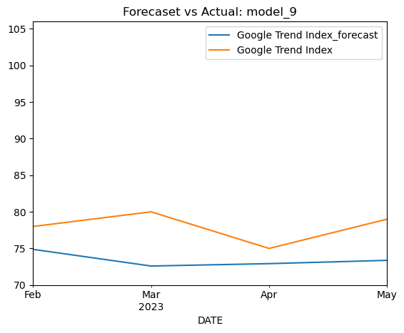
model_10 = build_VAR('model_10')
model_10
['Google Trend Index', 'CPI', 'Unemployment Rate']
 VAR Order Selection (* highlights the minimums)
=================================================
      AIC         BIC         FPE         HQIC
-------------------------------------------------
0    -0.8922*    -0.7797*     0.4097*    -0.8491*
1     -0.7163     -0.2660      0.4890     -0.5436
2     -0.8194    -0.03140      0.4429     -0.5173
3     -0.6123      0.5134      0.5501     -0.1807
4     -0.7255      0.7380      0.5001     -0.1644
5     -0.5685       1.233      0.6025      0.1220
6     -0.6837       1.455      0.5613      0.1363
7     -0.7234       1.753      0.5751      0.2260
-------------------------------------------------
  Summary of Regression Results
==================================
Model:                         VAR
Method:                        OLS
Date:           Mon, 22, Jul, 2024
Time:                     22:52:01
--------------------------------------------------------------------
No. of Equations:         3.00000    BIC:                  -0.526247
Nobs:                     58.0000    HQIC:                 -0.786493
Log likelihood:          -207.271    FPE:                   0.386012
AIC:                    -0.952545    Det(Omega_mle):        0.316016
--------------------------------------------------------------------
Results for equation Google Trend Index
========================================================================================
                           coefficient       std. error           t-stat            prob
----------------------------------------------------------------------------------------
const                        -0.079943         1.024976           -0.078           0.938
L1.Google Trend Index         0.167554         0.158697            1.056           0.291
L1.CPI                       30.470462        19.476949            1.564           0.118
L1.Unemployment Rate          1.153774         0.843426            1.368           0.171
========================================================================================

Results for equation CPI
========================================================================================
                           coefficient       std. error           t-stat            prob
----------------------------------------------------------------------------------------
const                         0.001848         0.007988            0.231           0.817
L1.Google Trend Index         0.000930         0.001237            0.752           0.452
L1.CPI                       -0.105645         0.151789           -0.696           0.486
L1.Unemployment Rate          0.009006         0.006573            1.370           0.171
========================================================================================

Results for equation Unemployment Rate
========================================================================================
                           coefficient       std. error           t-stat            prob
----------------------------------------------------------------------------------------
const                        -0.027577         0.190445           -0.145           0.885
L1.Google Trend Index        -0.029220         0.029487           -0.991           0.322
L1.CPI                       -4.851203         3.618910           -1.341           0.180
L1.Unemployment Rate         -0.105895         0.156712           -0.676           0.499
========================================================================================

Correlation matrix of residuals
                      Google Trend Index       CPI  Unemployment Rate
Google Trend Index              1.000000  0.304553          -0.507113
CPI                             0.304553  1.000000          -0.207440
Unemployment Rate              -0.507113 -0.207440           1.000000


/// The Durbin Watson Test ///
Google Trend Index : 1.99
CPI : 1.96
Unemployment Rate : 2.01
/Users/wakanamorlan/anaconda3/envs/py310/lib/python3.10/site-packages/statsmodels/tsa/base/tsa_model.py:471: ValueWarning: No frequency information was provided, so inferred frequency MS will be used.
  self._init_dates(dates, freq)
| RMSE | MAE | MSE | MAPE | Model_name | |
|---|---|---|---|---|---|
| 0 | 5.756 | 5.445 | 33.128 | 0.065 | model_10 |
model_11 = build_VAR('model_11')
model_11
['Google Trend Index', 'Visitor Volume', 'Average Daily Room Rate (ADR)', 'CPI']
 VAR Order Selection (* highlights the minimums)
=================================================
      AIC         BIC         FPE         HQIC
-------------------------------------------------
0      -4.730     -4.579*    0.008831      -4.672
1      -4.908      -4.157    0.007406      -4.620
2      -5.209      -3.858   0.005545*     -4.691*
3      -5.224      -3.273    0.005623      -4.476
4     -5.272*      -2.720    0.005674      -4.293
5      -5.023      -1.871    0.008000      -3.815
6      -4.980      -1.227    0.009715      -3.541
7      -4.639     -0.2867     0.01716      -2.971
-------------------------------------------------
  Summary of Regression Results
==================================
Model:                         VAR
Method:                        OLS
Date:           Mon, 22, Jul, 2024
Time:                     22:52:01
--------------------------------------------------------------------
No. of Equations:         4.00000    BIC:                   -2.92986
Nobs:                     55.0000    HQIC:                  -4.45192
Log likelihood:          -95.3460    FPE:                 0.00485347
AIC:                     -5.41165    Det(Omega_mle):      0.00165262
--------------------------------------------------------------------
Results for equation Google Trend Index
===================================================================================================
                                      coefficient       std. error           t-stat            prob
---------------------------------------------------------------------------------------------------
const                                    0.497680         0.960302            0.518           0.604
L1.Google Trend Index                   -0.018613         0.188724           -0.099           0.921
L1.Visitor Volume                        8.234046         3.075420            2.677           0.007
L1.Average Daily Room Rate (ADR)        -9.299647         2.737860           -3.397           0.001
L1.CPI                                  32.968449        22.525220            1.464           0.143
L2.Google Trend Index                   -0.526858         0.186446           -2.826           0.005
L2.Visitor Volume                        3.157082         4.180591            0.755           0.450
L2.Average Daily Room Rate (ADR)        -5.063769         3.501828           -1.446           0.148
L2.CPI                                  44.725820        24.067186            1.858           0.063
L3.Google Trend Index                   -0.095760         0.187265           -0.511           0.609
L3.Visitor Volume                        3.535340         4.089936            0.864           0.387
L3.Average Daily Room Rate (ADR)        -3.409416         3.181365           -1.072           0.284
L3.CPI                                   3.969567        26.366254            0.151           0.880
L4.Google Trend Index                   -0.054953         0.193019           -0.285           0.776
L4.Visitor Volume                        2.321468         3.673216            0.632           0.527
L4.Average Daily Room Rate (ADR)        -1.745734         2.573725           -0.678           0.498
L4.CPI                                  35.157998        25.530686            1.377           0.168
===================================================================================================

Results for equation Visitor Volume
===================================================================================================
                                      coefficient       std. error           t-stat            prob
---------------------------------------------------------------------------------------------------
const                                    0.035329         0.058545            0.603           0.546
L1.Google Trend Index                    0.009593         0.011506            0.834           0.404
L1.Visitor Volume                        0.545056         0.187493            2.907           0.004
L1.Average Daily Room Rate (ADR)        -0.417212         0.166914           -2.500           0.012
L1.CPI                                   0.423159         1.373251            0.308           0.758
L2.Google Trend Index                   -0.025126         0.011367           -2.210           0.027
L2.Visitor Volume                        0.257264         0.254870            1.009           0.313
L2.Average Daily Room Rate (ADR)        -0.177784         0.213489           -0.833           0.405
L2.CPI                                  -0.213579         1.467257           -0.146           0.884
L3.Google Trend Index                    0.009393         0.011417            0.823           0.411
L3.Visitor Volume                       -0.101979         0.249343           -0.409           0.683
L3.Average Daily Room Rate (ADR)        -0.185496         0.193952           -0.956           0.339
L3.CPI                                  -1.578148         1.607420           -0.982           0.326
L4.Google Trend Index                    0.008568         0.011767            0.728           0.467
L4.Visitor Volume                       -0.078221         0.223938           -0.349           0.727
L4.Average Daily Room Rate (ADR)        -0.247974         0.156907           -1.580           0.114
L4.CPI                                   1.804469         1.556479            1.159           0.246
===================================================================================================

Results for equation Average Daily Room Rate (ADR)
===================================================================================================
                                      coefficient       std. error           t-stat            prob
---------------------------------------------------------------------------------------------------
const                                    0.096087         0.061460            1.563           0.118
L1.Google Trend Index                   -0.002855         0.012079           -0.236           0.813
L1.Visitor Volume                        1.039794         0.196830            5.283           0.000
L1.Average Daily Room Rate (ADR)        -0.945826         0.175226           -5.398           0.000
L1.CPI                                  -0.055946         1.441638           -0.039           0.969
L2.Google Trend Index                   -0.000156         0.011933           -0.013           0.990
L2.Visitor Volume                        0.518393         0.267562            1.937           0.053
L2.Average Daily Room Rate (ADR)        -0.373045         0.224121           -1.664           0.096
L2.CPI                                  -4.607389         1.540325           -2.991           0.003
L3.Google Trend Index                    0.030349         0.011985            2.532           0.011
L3.Visitor Volume                       -0.302391         0.261760           -1.155           0.248
L3.Average Daily Room Rate (ADR)        -0.071878         0.203611           -0.353           0.724
L3.CPI                                  -5.979894         1.687468           -3.544           0.000
L4.Google Trend Index                    0.009193         0.012353            0.744           0.457
L4.Visitor Volume                       -0.294698         0.235090           -1.254           0.210
L4.Average Daily Room Rate (ADR)         0.066106         0.164721            0.401           0.688
L4.CPI                                  -0.885135         1.633991           -0.542           0.588
===================================================================================================

Results for equation CPI
===================================================================================================
                                      coefficient       std. error           t-stat            prob
---------------------------------------------------------------------------------------------------
const                                    0.001791         0.007265            0.247           0.805
L1.Google Trend Index                    0.001733         0.001428            1.214           0.225
L1.Visitor Volume                        0.014135         0.023265            0.608           0.543
L1.Average Daily Room Rate (ADR)        -0.019162         0.020712           -0.925           0.355
L1.CPI                                  -0.210811         0.170402           -1.237           0.216
L2.Google Trend Index                   -0.001354         0.001410           -0.960           0.337
L2.Visitor Volume                       -0.032108         0.031626           -1.015           0.310
L2.Average Daily Room Rate (ADR)        -0.002498         0.026491           -0.094           0.925
L2.CPI                                  -0.540169         0.182067           -2.967           0.003
L3.Google Trend Index                    0.001989         0.001417            1.404           0.160
L3.Visitor Volume                        0.027399         0.030940            0.886           0.376
L3.Average Daily Room Rate (ADR)        -0.007187         0.024067           -0.299           0.765
L3.CPI                                  -0.224152         0.199459           -1.124           0.261
L4.Google Trend Index                   -0.000605         0.001460           -0.414           0.679
L4.Visitor Volume                       -0.070388         0.027788           -2.533           0.011
L4.Average Daily Room Rate (ADR)         0.020557         0.019470            1.056           0.291
L4.CPI                                  -0.041392         0.193138           -0.214           0.830
===================================================================================================

Correlation matrix of residuals
                                 Google Trend Index  Visitor Volume  Average Daily Room Rate (ADR)       CPI
Google Trend Index                         1.000000        0.511815                       0.318084  0.462125
Visitor Volume                             0.511815        1.000000                       0.388557  0.377018
Average Daily Room Rate (ADR)              0.318084        0.388557                       1.000000  0.291263
CPI                                        0.462125        0.377018                       0.291263  1.000000


/// The Durbin Watson Test ///
Google Trend Index : 1.9
Visitor Volume : 1.9
Average Daily Room Rate (ADR) : 2.01
CPI : 2.0
/Users/wakanamorlan/anaconda3/envs/py310/lib/python3.10/site-packages/statsmodels/tsa/base/tsa_model.py:471: ValueWarning: No frequency information was provided, so inferred frequency MS will be used.
  self._init_dates(dates, freq)
| RMSE | MAE | MSE | MAPE | Model_name | |
|---|---|---|---|---|---|
| 0 | 2.496 | 1.891 | 6.229 | 0.024 | model_11 |
model_12 = build_VAR('model_12')
model_12
['Google Trend Index', 'Visitor Volume', 'Average Daily Room Rate (ADR)', 'Unemployment Rate']
VAR Order Selection (* highlights the minimums)
=================================================
AIC BIC FPE HQIC
-------------------------------------------------
0 1.129 1.279 3.092 1.186
1 0.4569 1.207* 1.583 0.7446*
2 0.4451 1.796 1.583* 0.9630
3 0.6300 2.581 1.961 1.378
4 0.7747 3.326 2.397 1.753
5 0.7110 3.863 2.475 1.919
6 0.6830 4.435 2.797 2.122
7 0.1346* 4.487 2.032 1.803
-------------------------------------------------
Summary of Regression Results
==================================
Model: VAR
Method: OLS
Date: Mon, 22, Jul, 2024
Time: 22:52:01
--------------------------------------------------------------------
No. of Equations: 4.00000 BIC: 4.48740
Nobs: 52.0000 HQIC: 1.80338
Log likelihood: -182.639 FPE: 2.03177
AIC: 0.134625 Det(Omega_mle): 0.345102
--------------------------------------------------------------------
Results for equation Google Trend Index
===================================================================================================
coefficient std. error t-stat prob
---------------------------------------------------------------------------------------------------
const 0.568046 0.922359 0.616 0.538
L1.Google Trend Index -0.048212 0.204711 -0.236 0.814
L1.Visitor Volume 10.021370 3.401338 2.946 0.003
L1.Average Daily Room Rate (ADR) -8.475508 2.765309 -3.065 0.002
L1.Unemployment Rate 0.847350 1.490500 0.569 0.570
L2.Google Trend Index -0.266175 0.234812 -1.134 0.257
L2.Visitor Volume 6.900590 6.928108 0.996 0.319
L2.Average Daily Room Rate (ADR) -6.651785 3.953290 -1.683 0.092
L2.Unemployment Rate -0.945486 1.525532 -0.620 0.535
L3.Google Trend Index -0.237942 0.246089 -0.967 0.334
L3.Visitor Volume -5.255417 6.398422 -0.821 0.411
L3.Average Daily Room Rate (ADR) 1.242070 3.696266 0.336 0.737
L3.Unemployment Rate -0.027928 1.602858 -0.017 0.986
L4.Google Trend Index 0.212802 0.253337 0.840 0.401
L4.Visitor Volume 4.850343 5.723409 0.847 0.397
L4.Average Daily Room Rate (ADR) -1.783217 3.733042 -0.478 0.633
L4.Unemployment Rate -0.080515 1.547731 -0.052 0.959
L5.Google Trend Index -0.321030 0.266823 -1.203 0.229
L5.Visitor Volume -3.056108 5.331236 -0.573 0.566
L5.Average Daily Room Rate (ADR) 4.917961 3.601563 1.366 0.172
L5.Unemployment Rate -2.258463 1.494830 -1.511 0.131
L6.Google Trend Index 0.062888 0.258065 0.244 0.807
L6.Visitor Volume -11.990933 5.757342 -2.083 0.037
L6.Average Daily Room Rate (ADR) 2.301988 3.580243 0.643 0.520
L6.Unemployment Rate 0.101251 1.500565 0.067 0.946
L7.Google Trend Index -0.069739 0.245616 -0.284 0.776
L7.Visitor Volume 7.477447 5.419084 1.380 0.168
L7.Average Daily Room Rate (ADR) -7.886631 3.470501 -2.272 0.023
L7.Unemployment Rate -3.040850 0.991680 -3.066 0.002
===================================================================================================
Results for equation Visitor Volume
===================================================================================================
coefficient std. error t-stat prob
---------------------------------------------------------------------------------------------------
const 0.087064 0.073565 1.184 0.237
L1.Google Trend Index 0.026151 0.016327 1.602 0.109
L1.Visitor Volume 0.565890 0.271281 2.086 0.037
L1.Average Daily Room Rate (ADR) -0.583703 0.220553 -2.647 0.008
L1.Unemployment Rate 0.073512 0.118878 0.618 0.536
L2.Google Trend Index -0.023840 0.018728 -1.273 0.203
L2.Visitor Volume 0.443935 0.552566 0.803 0.422
L2.Average Daily Room Rate (ADR) -0.539805 0.315303 -1.712 0.087
L2.Unemployment Rate -0.158889 0.121672 -1.306 0.192
L3.Google Trend Index 0.012853 0.019627 0.655 0.513
L3.Visitor Volume -0.444179 0.510320 -0.870 0.384
L3.Average Daily Room Rate (ADR) -0.197004 0.294803 -0.668 0.504
L3.Unemployment Rate 0.007339 0.127839 0.057 0.954
L4.Google Trend Index 0.023018 0.020205 1.139 0.255
L4.Visitor Volume 0.155625 0.456483 0.341 0.733
L4.Average Daily Room Rate (ADR) -0.464936 0.297737 -1.562 0.118
L4.Unemployment Rate 0.006418 0.123443 0.052 0.959
L5.Google Trend Index 0.005674 0.021281 0.267 0.790
L5.Visitor Volume -0.045887 0.425204 -0.108 0.914
L5.Average Daily Room Rate (ADR) 0.102329 0.287250 0.356 0.722
L5.Unemployment Rate 0.068921 0.119223 0.578 0.563
L6.Google Trend Index 0.005930 0.020583 0.288 0.773
L6.Visitor Volume 0.168260 0.459189 0.366 0.714
L6.Average Daily Room Rate (ADR) -0.180293 0.285550 -0.631 0.528
L6.Unemployment Rate 0.139096 0.119681 1.162 0.245
L7.Google Trend Index -0.004731 0.019590 -0.242 0.809
L7.Visitor Volume 0.829279 0.432210 1.919 0.055
L7.Average Daily Room Rate (ADR) -0.485877 0.276797 -1.755 0.079
L7.Unemployment Rate -0.035442 0.079094 -0.448 0.654
===================================================================================================
Results for equation Average Daily Room Rate (ADR)
===================================================================================================
coefficient std. error t-stat prob
---------------------------------------------------------------------------------------------------
const 0.182242 0.072749 2.505 0.012
L1.Google Trend Index -0.005470 0.016146 -0.339 0.735
L1.Visitor Volume 1.067918 0.268271 3.981 0.000
L1.Average Daily Room Rate (ADR) -1.163601 0.218106 -5.335 0.000
L1.Unemployment Rate -0.111910 0.117559 -0.952 0.341
L2.Google Trend Index 0.000742 0.018520 0.040 0.968
L2.Visitor Volume 0.330468 0.546436 0.605 0.545
L2.Average Daily Room Rate (ADR) -0.563254 0.311805 -1.806 0.071
L2.Unemployment Rate 0.173456 0.120322 1.442 0.149
L3.Google Trend Index 0.013307 0.019410 0.686 0.493
L3.Visitor Volume 0.647251 0.504658 1.283 0.200
L3.Average Daily Room Rate (ADR) -0.651575 0.291533 -2.235 0.025
L3.Unemployment Rate 0.186109 0.126421 1.472 0.141
L4.Google Trend Index -0.016566 0.019981 -0.829 0.407
L4.Visitor Volume 0.817092 0.451419 1.810 0.070
L4.Average Daily Room Rate (ADR) -0.390790 0.294434 -1.327 0.184
L4.Unemployment Rate 0.096527 0.122073 0.791 0.429
L5.Google Trend Index -0.012996 0.021045 -0.618 0.537
L5.Visitor Volume 0.453867 0.420487 1.079 0.280
L5.Average Daily Room Rate (ADR) -0.178078 0.284064 -0.627 0.531
L5.Unemployment Rate 0.152972 0.117901 1.297 0.194
L6.Google Trend Index -0.016618 0.020354 -0.816 0.414
L6.Visitor Volume 0.949461 0.454095 2.091 0.037
L6.Average Daily Room Rate (ADR) -0.290698 0.282382 -1.029 0.303
L6.Unemployment Rate 0.309695 0.118353 2.617 0.009
L7.Google Trend Index -0.026285 0.019372 -1.357 0.175
L7.Visitor Volume 1.360576 0.427416 3.183 0.001
L7.Average Daily Room Rate (ADR) -0.424751 0.273726 -1.552 0.121
L7.Unemployment Rate 0.040037 0.078216 0.512 0.609
===================================================================================================
Results for equation Unemployment Rate
===================================================================================================
coefficient std. error t-stat prob
---------------------------------------------------------------------------------------------------
const -0.128207 0.140780 -0.911 0.362
L1.Google Trend Index 0.054713 0.031245 1.751 0.080
L1.Visitor Volume -4.340606 0.519148 -8.361 0.000
L1.Average Daily Room Rate (ADR) 2.019122 0.422071 4.784 0.000
L1.Unemployment Rate -0.079559 0.227496 -0.350 0.727
L2.Google Trend Index 0.075742 0.035840 2.113 0.035
L2.Visitor Volume -0.166068 1.057442 -0.157 0.875
L2.Average Daily Room Rate (ADR) 0.210501 0.603393 0.349 0.727
L2.Unemployment Rate -0.042670 0.232843 -0.183 0.855
L3.Google Trend Index -0.025844 0.037561 -0.688 0.491
L3.Visitor Volume -0.239841 0.976596 -0.246 0.806
L3.Average Daily Room Rate (ADR) 0.637773 0.564164 1.130 0.258
L3.Unemployment Rate -0.284552 0.244645 -1.163 0.245
L4.Google Trend Index 0.033261 0.038667 0.860 0.390
L4.Visitor Volume -1.126027 0.873568 -1.289 0.197
L4.Average Daily Room Rate (ADR) 0.268252 0.569777 0.471 0.638
L4.Unemployment Rate -0.216014 0.236231 -0.914 0.360
L5.Google Trend Index 0.033429 0.040725 0.821 0.412
L5.Visitor Volume -0.981981 0.813710 -1.207 0.228
L5.Average Daily Room Rate (ADR) -0.527426 0.549709 -0.959 0.337
L5.Unemployment Rate -0.105056 0.228157 -0.460 0.645
L6.Google Trend Index 0.025842 0.039389 0.656 0.512
L6.Visitor Volume 0.380920 0.878747 0.433 0.665
L6.Average Daily Room Rate (ADR) 0.191724 0.546455 0.351 0.726
L6.Unemployment Rate -0.075174 0.229032 -0.328 0.743
L7.Google Trend Index -0.028878 0.037489 -0.770 0.441
L7.Visitor Volume -0.568752 0.827119 -0.688 0.492
L7.Average Daily Room Rate (ADR) 0.091077 0.529705 0.172 0.863
L7.Unemployment Rate -0.095745 0.151361 -0.633 0.527
===================================================================================================
Correlation matrix of residuals
Google Trend Index Visitor Volume Average Daily Room Rate (ADR) Unemployment Rate
Google Trend Index 1.000000 0.586632 0.382448 -0.532869
Visitor Volume 0.586632 1.000000 0.494676 -0.420493
Average Daily Room Rate (ADR) 0.382448 0.494676 1.000000 -0.370968
Unemployment Rate -0.532869 -0.420493 -0.370968 1.000000
/// The Durbin Watson Test ///
Google Trend Index : 1.79
Visitor Volume : 1.83
Average Daily Room Rate (ADR) : 2.02
Unemployment Rate : 1.82
/Users/wakanamorlan/anaconda3/envs/py310/lib/python3.10/site-packages/statsmodels/tsa/base/tsa_model.py:471: ValueWarning: No frequency information was provided, so inferred frequency MS will be used.
  self._init_dates(dates, freq)
| RMSE | MAE | MSE | MAPE | Model_name | |
|---|---|---|---|---|---|
| 0 | 9.633 | 8.704 | 92.797 | 0.111 | model_12 |
model_13 = build_VAR('model_13')
model_13
['Google Trend Index', 'Visitor Volume', 'CPI', 'Unemployment Rate']
VAR Order Selection (* highlights the minimums)
=================================================
AIC BIC FPE HQIC
-------------------------------------------------
0 -2.968 -2.818* 0.05140 -2.911
1 -3.290 -2.539 0.03735* -3.002*
2 -3.287 -1.937 0.03788 -2.770
3 -3.120 -1.169 0.04611 -2.372
4 -3.236 -0.6845 0.04344 -2.258
5 -3.428 -0.2763 0.03943 -2.220
6 -3.511 0.2419 0.04222 -2.072
7 -3.554* 0.7984 0.05079 -1.886
-------------------------------------------------
Summary of Regression Results
==================================
Model: VAR
Method: OLS
Date: Mon, 22, Jul, 2024
Time: 22:52:01
--------------------------------------------------------------------
No. of Equations: 4.00000 BIC: 0.798364
Nobs: 52.0000 HQIC: -1.88566
Log likelihood: -86.7245 FPE: 0.0507863
AIC: -3.55441 Det(Omega_mle): 0.00862620
--------------------------------------------------------------------
Results for equation Google Trend Index
========================================================================================
coefficient std. error t-stat prob
----------------------------------------------------------------------------------------
const -0.105612 1.063420 -0.099 0.921
L1.Google Trend Index -0.192392 0.284634 -0.676 0.499
L1.Visitor Volume 8.022198 4.153194 1.932 0.053
L1.CPI -9.414886 38.996331 -0.241 0.809
L1.Unemployment Rate 0.658787 1.692331 0.389 0.697
L2.Google Trend Index -0.135574 0.352505 -0.385 0.701
L2.Visitor Volume -1.009166 6.635058 -0.152 0.879
L2.CPI -15.941374 39.317201 -0.405 0.685
L2.Unemployment Rate 0.753767 1.695796 0.444 0.657
L3.Google Trend Index -0.215047 0.286871 -0.750 0.453
L3.Visitor Volume -1.112003 6.273196 -0.177 0.859
L3.CPI -24.170261 41.056381 -0.589 0.556
L3.Unemployment Rate -0.860927 1.707328 -0.504 0.614
L4.Google Trend Index -0.122688 0.294635 -0.416 0.677
L4.Visitor Volume 0.744147 6.076902 0.122 0.903
L4.CPI 19.702734 38.279075 0.515 0.607
L4.Unemployment Rate -0.981174 1.701076 -0.577 0.564
L5.Google Trend Index -0.053924 0.291345 -0.185 0.853
L5.Visitor Volume -0.661969 7.784941 -0.085 0.932
L5.CPI -27.908383 40.529388 -0.689 0.491
L5.Unemployment Rate -2.282030 1.974952 -1.155 0.248
L6.Google Trend Index 0.023437 0.341437 0.069 0.945
L6.Visitor Volume -13.435544 9.073423 -1.481 0.139
L6.CPI -20.235593 34.128670 -0.593 0.553
L6.Unemployment Rate -3.546873 1.920606 -1.847 0.065
L7.Google Trend Index 0.257790 0.308239 0.836 0.403
L7.Visitor Volume -8.787663 7.593294 -1.157 0.247
L7.CPI -32.812978 39.976091 -0.821 0.412
L7.Unemployment Rate -3.098254 1.335608 -2.320 0.020
========================================================================================
Results for equation Visitor Volume
========================================================================================
coefficient std. error t-stat prob
----------------------------------------------------------------------------------------
const 0.000843 0.072250 0.012 0.991
L1.Google Trend Index 0.016456 0.019338 0.851 0.395
L1.Visitor Volume 0.452930 0.282173 1.605 0.108
L1.CPI 0.708547 2.649461 0.267 0.789
L1.Unemployment Rate 0.079175 0.114979 0.689 0.491
L2.Google Trend Index -0.020561 0.023950 -0.859 0.391
L2.Visitor Volume 0.042480 0.450794 0.094 0.925
L2.CPI -1.869894 2.671262 -0.700 0.484
L2.Unemployment Rate -0.091484 0.115215 -0.794 0.427
L3.Google Trend Index 0.020192 0.019490 1.036 0.300
L3.Visitor Volume -0.511444 0.426209 -1.200 0.230
L3.CPI -2.483227 2.789424 -0.890 0.373
L3.Unemployment Rate -0.129085 0.115998 -1.113 0.266
L4.Google Trend Index 0.011502 0.020018 0.575 0.566
L4.Visitor Volume -0.637588 0.412873 -1.544 0.123
L4.CPI 1.899398 2.600730 0.730 0.465
L4.Unemployment Rate -0.013035 0.115573 -0.113 0.910
L5.Google Trend Index 0.024914 0.019794 1.259 0.208
L5.Visitor Volume 0.182127 0.528919 0.344 0.731
L5.CPI -1.831945 2.753619 -0.665 0.506
L5.Unemployment Rate 0.033670 0.134181 0.251 0.802
L6.Google Trend Index -0.001907 0.023198 -0.082 0.934
L6.Visitor Volume -0.244439 0.616460 -0.397 0.692
L6.CPI -0.592423 2.318746 -0.255 0.798
L6.Unemployment Rate -0.122649 0.130488 -0.940 0.347
L7.Google Trend Index 0.022854 0.020942 1.091 0.275
L7.Visitor Volume -0.517525 0.515898 -1.003 0.316
L7.CPI -0.978279 2.716027 -0.360 0.719
L7.Unemployment Rate -0.088057 0.090743 -0.970 0.332
========================================================================================
Results for equation CPI
========================================================================================
coefficient std. error t-stat prob
----------------------------------------------------------------------------------------
const 0.001478 0.007204 0.205 0.837
L1.Google Trend Index 0.002413 0.001928 1.252 0.211
L1.Visitor Volume 0.002811 0.028133 0.100 0.920
L1.CPI -0.233224 0.264157 -0.883 0.377
L1.Unemployment Rate 0.005865 0.011464 0.512 0.609
L2.Google Trend Index -0.001224 0.002388 -0.513 0.608
L2.Visitor Volume -0.017539 0.044945 -0.390 0.696
L2.CPI -0.450655 0.266331 -1.692 0.091
L2.Unemployment Rate -0.001538 0.011487 -0.134 0.894
L3.Google Trend Index 0.001344 0.001943 0.692 0.489
L3.Visitor Volume 0.009871 0.042494 0.232 0.816
L3.CPI -0.205795 0.278112 -0.740 0.459
L3.Unemployment Rate -0.007530 0.011565 -0.651 0.515
L4.Google Trend Index 0.000696 0.001996 0.349 0.727
L4.Visitor Volume -0.100277 0.041164 -2.436 0.015
L4.CPI -0.071822 0.259299 -0.277 0.782
L4.Unemployment Rate -0.014542 0.011523 -1.262 0.207
L5.Google Trend Index 0.000773 0.001974 0.392 0.695
L5.Visitor Volume -0.018197 0.052734 -0.345 0.730
L5.CPI 0.024863 0.274542 0.091 0.928
L5.Unemployment Rate -0.005180 0.013378 -0.387 0.699
L6.Google Trend Index -0.001458 0.002313 -0.631 0.528
L6.Visitor Volume 0.029327 0.061462 0.477 0.633
L6.CPI -0.492447 0.231184 -2.130 0.033
L6.Unemployment Rate -0.009950 0.013010 -0.765 0.444
L7.Google Trend Index 0.002291 0.002088 1.097 0.273
L7.Visitor Volume -0.032437 0.051436 -0.631 0.528
L7.CPI -0.000448 0.270794 -0.002 0.999
L7.Unemployment Rate 0.004732 0.009047 0.523 0.601
========================================================================================
Results for equation Unemployment Rate
========================================================================================
coefficient std. error t-stat prob
----------------------------------------------------------------------------------------
const -0.025837 0.168989 -0.153 0.878
L1.Google Trend Index 0.090825 0.045231 2.008 0.045
L1.Visitor Volume -3.747108 0.659987 -5.678 0.000
L1.CPI -5.494987 6.196936 -0.887 0.375
L1.Unemployment Rate -0.525865 0.268930 -1.955 0.051
L2.Google Trend Index 0.064961 0.056017 1.160 0.246
L2.Visitor Volume -0.858620 1.054382 -0.814 0.415
L2.CPI 5.272241 6.247926 0.844 0.399
L2.Unemployment Rate -0.049630 0.269480 -0.184 0.854
L3.Google Trend Index 0.007989 0.045587 0.175 0.861
L3.Visitor Volume 0.791389 0.996878 0.794 0.427
L3.CPI 2.091567 6.524301 0.321 0.749
L3.Unemployment Rate 0.086823 0.271313 0.320 0.749
L4.Google Trend Index 0.014626 0.046821 0.312 0.755
L4.Visitor Volume -0.005844 0.965685 -0.006 0.995
L4.CPI -2.549514 6.082957 -0.419 0.675
L4.Unemployment Rate -0.450615 0.270319 -1.667 0.096
L5.Google Trend Index 0.045618 0.046298 0.985 0.324
L5.Visitor Volume -2.890343 1.237111 -2.336 0.019
L5.CPI 6.439078 6.440556 1.000 0.317
L5.Unemployment Rate 0.010262 0.313841 0.033 0.974
L6.Google Trend Index 0.015400 0.054258 0.284 0.777
L6.Visitor Volume 1.649292 1.441864 1.144 0.253
L6.CPI 5.481297 5.423413 1.011 0.312
L6.Unemployment Rate 0.421328 0.305205 1.380 0.167
L7.Google Trend Index -0.090749 0.048983 -1.853 0.064
L7.Visitor Volume 2.211603 1.206656 1.833 0.067
L7.CPI 4.035935 6.352631 0.635 0.525
L7.Unemployment Rate 0.187242 0.212243 0.882 0.378
========================================================================================
Correlation matrix of residuals
Google Trend Index Visitor Volume CPI Unemployment Rate
Google Trend Index 1.000000 0.693161 0.619344 -0.634892
Visitor Volume 0.693161 1.000000 0.483473 -0.473241
CPI 0.619344 0.483473 1.000000 -0.616666
Unemployment Rate -0.634892 -0.473241 -0.616666 1.000000
/// The Durbin Watson Test ///
Google Trend Index : 2.1
Visitor Volume : 2.13
CPI : 2.12
Unemployment Rate : 2.24
/Users/wakanamorlan/anaconda3/envs/py310/lib/python3.10/site-packages/statsmodels/tsa/base/tsa_model.py:471: ValueWarning: No frequency information was provided, so inferred frequency MS will be used.
  self._init_dates(dates, freq)
| RMSE | MAE | MSE | MAPE | Model_name | |
|---|---|---|---|---|---|
| 0 | 7.624 | 6.003 | 58.132 | 0.074 | model_13 |
model_14 = build_VAR('model_14')
model_14
['Google Trend Index', 'Average Daily Room Rate (ADR)', 'CPI', 'Unemployment Rate']
 VAR Order Selection (* highlights the minimums)
=================================================
      AIC         BIC         FPE         HQIC
-------------------------------------------------
0      -2.382     -2.232*     0.09237     -2.324*
1      -2.268      -1.518      0.1038      -1.980
2     -2.536*      -1.185    0.08028*      -2.018
3      -2.317     -0.3658      0.1029      -1.569
4      -2.026      0.5257      0.1457      -1.048
5      -1.696       1.456      0.2230     -0.4871
6      -1.716       2.037      0.2541     -0.2771
7      -1.835       2.518      0.2836     -0.1658
-------------------------------------------------
  Summary of Regression Results
==================================
Model:                         VAR
Method:                        OLS
Date:           Mon, 22, Jul, 2024
Time:                     22:52:01
--------------------------------------------------------------------
No. of Equations:         4.00000    BIC:                   -1.53568
Nobs:                     57.0000    HQIC:                  -2.32455
Log likelihood:          -206.976    FPE:                  0.0598827
AIC:                     -2.82602    Det(Omega_mle):       0.0333139
--------------------------------------------------------------------
Results for equation Google Trend Index
===================================================================================================
                                      coefficient       std. error           t-stat            prob
---------------------------------------------------------------------------------------------------
const                                    0.213965         0.946526            0.226           0.821
L1.Google Trend Index                    0.184843         0.155762            1.187           0.235
L1.Average Daily Room Rate (ADR)        -6.998566         2.248011           -3.113           0.002
L1.CPI                                  40.459134        19.379487            2.088           0.037
L1.Unemployment Rate                    -0.416368         0.892125           -0.467           0.641
L2.Google Trend Index                   -0.281786         0.152684           -1.846           0.065
L2.Average Daily Room Rate (ADR)        -2.101772         2.365946           -0.888           0.374
L2.CPI                                  24.668523        19.709846            1.252           0.211
L2.Unemployment Rate                    -0.067173         0.953953           -0.070           0.944
===================================================================================================

Results for equation Average Daily Room Rate (ADR)
===================================================================================================
                                      coefficient       std. error           t-stat            prob
---------------------------------------------------------------------------------------------------
const                                    0.053563         0.073171            0.732           0.464
L1.Google Trend Index                   -0.000830         0.012041           -0.069           0.945
L1.Average Daily Room Rate (ADR)        -0.409542         0.173782           -2.357           0.018
L1.CPI                                   2.204655         1.498130            1.472           0.141
L1.Unemployment Rate                    -0.126539         0.068966           -1.835           0.067
L2.Google Trend Index                    0.020829         0.011803            1.765           0.078
L2.Average Daily Room Rate (ADR)        -0.052791         0.182899           -0.289           0.773
L2.CPI                                  -2.386846         1.523668           -1.567           0.117
L2.Unemployment Rate                     0.117207         0.073745            1.589           0.112
===================================================================================================

Results for equation CPI
===================================================================================================
                                      coefficient       std. error           t-stat            prob
---------------------------------------------------------------------------------------------------
const                                    0.001302         0.007399            0.176           0.860
L1.Google Trend Index                    0.001187         0.001218            0.975           0.329
L1.Average Daily Room Rate (ADR)        -0.000773         0.017572           -0.044           0.965
L1.CPI                                  -0.183323         0.151486           -1.210           0.226
L1.Unemployment Rate                     0.005866         0.006974            0.841           0.400
L2.Google Trend Index                   -0.000751         0.001194           -0.629           0.529
L2.Average Daily Room Rate (ADR)        -0.018652         0.018494           -1.009           0.313
L2.CPI                                  -0.423560         0.154068           -2.749           0.006
L2.Unemployment Rate                    -0.001043         0.007457           -0.140           0.889
===================================================================================================

Results for equation Unemployment Rate
===================================================================================================
                                      coefficient       std. error           t-stat            prob
---------------------------------------------------------------------------------------------------
const                                   -0.013302         0.195481           -0.068           0.946
L1.Google Trend Index                   -0.047594         0.032169           -1.480           0.139
L1.Average Daily Room Rate (ADR)         0.549426         0.464269            1.183           0.237
L1.CPI                                  -4.721153         4.002335           -1.180           0.238
L1.Unemployment Rate                     0.031360         0.184245            0.170           0.865
L2.Google Trend Index                    0.016397         0.031533            0.520           0.603
L2.Average Daily Room Rate (ADR)        -0.660045         0.488625           -1.351           0.177
L2.CPI                                   0.492523         4.070562            0.121           0.904
L2.Unemployment Rate                    -0.169937         0.197014           -0.863           0.388
===================================================================================================

Correlation matrix of residuals
                                 Google Trend Index  Average Daily Room Rate (ADR)       CPI  Unemployment Rate
Google Trend Index                         1.000000                       0.445387  0.342082          -0.514851
Average Daily Room Rate (ADR)              0.445387                       1.000000  0.354554          -0.647043
CPI                                        0.342082                       0.354554  1.000000          -0.284482
Unemployment Rate                         -0.514851                      -0.647043 -0.284482           1.000000


/// The Durbin Watson Test ///
Google Trend Index : 1.94
Average Daily Room Rate (ADR) : 2.26
CPI : 1.97
Unemployment Rate : 1.95
/Users/wakanamorlan/anaconda3/envs/py310/lib/python3.10/site-packages/statsmodels/tsa/base/tsa_model.py:471: ValueWarning: No frequency information was provided, so inferred frequency MS will be used.
  self._init_dates(dates, freq)
| RMSE | MAE | MSE | MAPE | Model_name | |
|---|---|---|---|---|---|
| 0 | 2.404 | 2.092 | 5.779 | 0.026 | model_14 |
model_15 = build_VAR('model_15')
model_15
['Google Trend Index', 'Visitor Volume', 'Average Daily Room Rate (ADR)', 'CPI', 'Unemployment Rate']
VAR Order Selection (* highlights the minimums)
=================================================
AIC BIC FPE HQIC
-------------------------------------------------
0 -4.523 -4.335* 0.01086 -4.451
1 -5.166 -4.040 0.005737 -4.734*
2 -5.337 -3.273 0.004969* -4.546
3 -5.296 -2.294 0.005555 -4.145
4 -5.324 -1.384 0.006221 -3.813
5 -5.596 -0.7179 0.006079 -3.726
6 -5.684 0.1321 0.008446 -3.454
7 -5.901* 0.8536 0.01357 -3.311
-------------------------------------------------
Summary of Regression Results
==================================
Model: VAR
Method: OLS
Date: Mon, 22, Jul, 2024
Time: 22:52:02
--------------------------------------------------------------------
No. of Equations: 5.00000 BIC: 0.853606
Nobs: 52.0000 HQIC: -3.31126
Log likelihood: -35.5058 FPE: 0.0135681
AIC: -5.90070 Det(Omega_mle): 0.000977511
--------------------------------------------------------------------
Results for equation Google Trend Index
===================================================================================================
coefficient std. error t-stat prob
---------------------------------------------------------------------------------------------------
const 0.526056 1.138175 0.462 0.644
L1.Google Trend Index -0.085840 0.267404 -0.321 0.748
L1.Visitor Volume 9.490544 3.937402 2.410 0.016
L1.Average Daily Room Rate (ADR) -8.818667 3.511345 -2.511 0.012
L1.CPI 4.514952 41.599508 0.109 0.914
L1.Unemployment Rate 1.519518 2.154528 0.705 0.481
L2.Google Trend Index -0.043030 0.331903 -0.130 0.897
L2.Visitor Volume 13.038984 10.923600 1.194 0.233
L2.Average Daily Room Rate (ADR) -10.219262 6.446754 -1.585 0.113
L2.CPI -62.759146 44.621175 -1.406 0.160
L2.Unemployment Rate -2.577151 2.073821 -1.243 0.214
L3.Google Trend Index -0.164418 0.316820 -0.519 0.604
L3.Visitor Volume -14.258844 10.133083 -1.407 0.159
L3.Average Daily Room Rate (ADR) 4.975288 5.728572 0.869 0.385
L3.CPI -44.086245 42.228901 -1.044 0.296
L3.Unemployment Rate -1.683471 2.226280 -0.756 0.450
L4.Google Trend Index 0.736317 0.428067 1.720 0.085
L4.Visitor Volume -1.834179 8.783384 -0.209 0.835
L4.Average Daily Room Rate (ADR) 0.686592 5.399698 0.127 0.899
L4.CPI -63.224493 43.858771 -1.442 0.149
L4.Unemployment Rate 0.814524 2.364963 0.344 0.731
L5.Google Trend Index -0.293587 0.350382 -0.838 0.402
L5.Visitor Volume -1.105943 10.787922 -0.103 0.918
L5.Average Daily Room Rate (ADR) 7.187579 5.005349 1.436 0.151
L5.CPI -30.937282 46.718487 -0.662 0.508
L5.Unemployment Rate -4.056879 2.326465 -1.744 0.081
L6.Google Trend Index 0.280103 0.337164 0.831 0.406
L6.Visitor Volume -25.281038 12.044977 -2.099 0.036
L6.Average Daily Room Rate (ADR) 7.428968 5.696322 1.304 0.192
L6.CPI -39.625420 42.454906 -0.933 0.351
L6.Unemployment Rate -0.953478 2.161694 -0.441 0.659
L7.Google Trend Index 0.069363 0.359535 0.193 0.847
L7.Visitor Volume 2.660708 9.427740 0.282 0.778
L7.Average Daily Room Rate (ADR) -8.626854 4.629597 -1.863 0.062
L7.CPI -13.338067 45.721953 -0.292 0.770
L7.Unemployment Rate -4.295594 1.451192 -2.960 0.003
===================================================================================================
Results for equation Visitor Volume
===================================================================================================
coefficient std. error t-stat prob
---------------------------------------------------------------------------------------------------
const 0.081373 0.092038 0.884 0.377
L1.Google Trend Index 0.029056 0.021624 1.344 0.179
L1.Visitor Volume 0.534506 0.318396 1.679 0.093
L1.Average Daily Room Rate (ADR) -0.627493 0.283943 -2.210 0.027
L1.CPI 2.331957 3.363923 0.693 0.488
L1.Unemployment Rate 0.153845 0.174225 0.883 0.377
L2.Google Trend Index -0.032585 0.026839 -1.214 0.225
L2.Visitor Volume 0.924992 0.883331 1.047 0.295
L2.Average Daily Room Rate (ADR) -0.664547 0.521314 -1.275 0.202
L2.CPI -1.411184 3.608269 -0.391 0.696
L2.Unemployment Rate -0.214942 0.167698 -1.282 0.200
L3.Google Trend Index 0.013896 0.025619 0.542 0.588
L3.Visitor Volume -0.674305 0.819407 -0.823 0.411
L3.Average Daily Room Rate (ADR) -0.031134 0.463238 -0.067 0.946
L3.CPI -1.990547 3.414819 -0.583 0.560
L3.Unemployment Rate -0.058042 0.180027 -0.322 0.747
L4.Google Trend Index 0.034778 0.034615 1.005 0.315
L4.Visitor Volume -0.276262 0.710264 -0.389 0.697
L4.Average Daily Room Rate (ADR) -0.295386 0.436644 -0.676 0.499
L4.CPI -0.804040 3.546617 -0.227 0.821
L4.Unemployment Rate 0.061976 0.191242 0.324 0.746
L5.Google Trend Index 0.002142 0.028333 0.076 0.940
L5.Visitor Volume 0.218430 0.872360 0.250 0.802
L5.Average Daily Room Rate (ADR) 0.146709 0.404755 0.362 0.717
L5.CPI 0.100327 3.777867 0.027 0.979
L5.Unemployment Rate 0.101391 0.188128 0.539 0.590
L6.Google Trend Index -0.000006 0.027265 -0.000 1.000
L6.Visitor Volume 0.169182 0.974011 0.174 0.862
L6.Average Daily Room Rate (ADR) -0.156955 0.460630 -0.341 0.733
L6.CPI -0.098528 3.433095 -0.029 0.977
L6.Unemployment Rate 0.102699 0.174804 0.588 0.557
L7.Google Trend Index -0.005931 0.029074 -0.204 0.838
L7.Visitor Volume 0.534996 0.762369 0.702 0.483
L7.Average Daily Room Rate (ADR) -0.585237 0.374370 -1.563 0.118
L7.CPI 1.879301 3.697283 0.508 0.611
L7.Unemployment Rate -0.093252 0.117350 -0.795 0.427
===================================================================================================
Results for equation Average Daily Room Rate (ADR)
===================================================================================================
coefficient std. error t-stat prob
---------------------------------------------------------------------------------------------------
const 0.143935 0.086902 1.656 0.098
L1.Google Trend Index -0.001991 0.020417 -0.097 0.922
L1.Visitor Volume 1.125590 0.300627 3.744 0.000
L1.Average Daily Room Rate (ADR) -1.166110 0.268097 -4.350 0.000
L1.CPI 0.298972 3.176192 0.094 0.925
L1.Unemployment Rate -0.107757 0.164502 -0.655 0.512
L2.Google Trend Index -0.007539 0.025341 -0.297 0.766
L2.Visitor Volume 0.431513 0.834035 0.517 0.605
L2.Average Daily Room Rate (ADR) -0.424483 0.492220 -0.862 0.388
L2.CPI -2.463004 3.406902 -0.723 0.470
L2.Unemployment Rate 0.070820 0.158340 0.447 0.655
L3.Google Trend Index 0.020591 0.024190 0.851 0.395
L3.Visitor Volume 0.167752 0.773678 0.217 0.828
L3.Average Daily Room Rate (ADR) -0.260237 0.437386 -0.595 0.552
L3.CPI -3.209335 3.224247 -0.995 0.320
L3.Unemployment Rate 0.098865 0.169980 0.582 0.561
L4.Google Trend Index -0.009837 0.032684 -0.301 0.763
L4.Visitor Volume 0.154125 0.670626 0.230 0.818
L4.Average Daily Room Rate (ADR) -0.014480 0.412276 -0.035 0.972
L4.CPI 1.216270 3.348691 0.363 0.716
L4.Unemployment Rate 0.147832 0.180569 0.819 0.413
L5.Google Trend Index -0.016778 0.026752 -0.627 0.531
L5.Visitor Volume 0.584322 0.823676 0.709 0.478
L5.Average Daily Room Rate (ADR) -0.140372 0.382167 -0.367 0.713
L5.CPI 1.490067 3.567035 0.418 0.676
L5.Unemployment Rate 0.169439 0.177629 0.954 0.340
L6.Google Trend Index -0.029924 0.025743 -1.162 0.245
L6.Visitor Volume 1.006541 0.919654 1.094 0.274
L6.Average Daily Room Rate (ADR) -0.368751 0.434924 -0.848 0.397
L6.CPI 2.108528 3.241503 0.650 0.515
L6.Unemployment Rate 0.197989 0.165049 1.200 0.230
L7.Google Trend Index -0.028620 0.027451 -1.043 0.297
L7.Visitor Volume 0.988868 0.719824 1.374 0.170
L7.Average Daily Room Rate (ADR) -0.470594 0.353478 -1.331 0.183
L7.CPI 0.971890 3.490948 0.278 0.781
L7.Unemployment Rate -0.051192 0.110801 -0.462 0.644
===================================================================================================
Results for equation CPI
===================================================================================================
coefficient std. error t-stat prob
---------------------------------------------------------------------------------------------------
const -0.001083 0.009285 -0.117 0.907
L1.Google Trend Index 0.002758 0.002182 1.264 0.206
L1.Visitor Volume 0.003602 0.032122 0.112 0.911
L1.Average Daily Room Rate (ADR) -0.018957 0.028646 -0.662 0.508
L1.CPI -0.239427 0.339376 -0.705 0.481
L1.Unemployment Rate -0.001386 0.017577 -0.079 0.937
L2.Google Trend Index 0.000216 0.002708 0.080 0.936
L2.Visitor Volume -0.017546 0.089117 -0.197 0.844
L2.Average Daily Room Rate (ADR) -0.002347 0.052594 -0.045 0.964
L2.CPI -0.759615 0.364027 -2.087 0.037
L2.Unemployment Rate -0.014577 0.016919 -0.862 0.389
L3.Google Trend Index 0.002741 0.002585 1.060 0.289
L3.Visitor Volume -0.067636 0.082667 -0.818 0.413
L3.Average Daily Room Rate (ADR) 0.036639 0.046735 0.784 0.433
L3.CPI -0.309435 0.344511 -0.898 0.369
L3.Unemployment Rate -0.021348 0.018162 -1.175 0.240
L4.Google Trend Index 0.003830 0.003492 1.097 0.273
L4.Visitor Volume -0.159807 0.071656 -2.230 0.026
L4.Average Daily Room Rate (ADR) 0.045703 0.044052 1.037 0.300
L4.CPI -0.346919 0.357807 -0.970 0.332
L4.Unemployment Rate -0.007691 0.019294 -0.399 0.690
L5.Google Trend Index 0.000999 0.002858 0.349 0.727
L5.Visitor Volume -0.028161 0.088010 -0.320 0.749
L5.Average Daily Room Rate (ADR) 0.028614 0.040834 0.701 0.483
L5.CPI 0.026948 0.381137 0.071 0.944
L5.Unemployment Rate -0.020509 0.018980 -1.081 0.280
L6.Google Trend Index -0.000942 0.002751 -0.343 0.732
L6.Visitor Volume -0.057913 0.098265 -0.589 0.556
L6.Average Daily Room Rate (ADR) 0.038365 0.046472 0.826 0.409
L6.CPI -0.422269 0.346354 -1.219 0.223
L6.Unemployment Rate -0.005122 0.017635 -0.290 0.771
L7.Google Trend Index 0.002668 0.002933 0.910 0.363
L7.Visitor Volume 0.002885 0.076913 0.038 0.970
L7.Average Daily Room Rate (ADR) -0.044039 0.037769 -1.166 0.244
L7.CPI 0.108452 0.373008 0.291 0.771
L7.Unemployment Rate -0.005314 0.011839 -0.449 0.654
===================================================================================================
Results for equation Unemployment Rate
===================================================================================================
coefficient std. error t-stat prob
---------------------------------------------------------------------------------------------------
const -0.088056 0.169741 -0.519 0.604
L1.Google Trend Index 0.063263 0.039879 1.586 0.113
L1.Visitor Volume -4.346137 0.587203 -7.401 0.000
L1.Average Daily Room Rate (ADR) 1.848416 0.523663 3.530 0.000
L1.CPI -3.104133 6.203928 -0.500 0.617
L1.Unemployment Rate -0.174021 0.321315 -0.542 0.588
L2.Google Trend Index 0.073314 0.049498 1.481 0.139
L2.Visitor Volume -0.770037 1.629087 -0.473 0.636
L2.Average Daily Room Rate (ADR) 0.335610 0.961434 0.349 0.727
L2.CPI 6.848556 6.654563 1.029 0.303
L2.Unemployment Rate 0.104475 0.309279 0.338 0.736
L3.Google Trend Index -0.045266 0.047249 -0.958 0.338
L3.Visitor Volume 0.631816 1.511194 0.418 0.676
L3.Average Daily Room Rate (ADR) 0.291467 0.854329 0.341 0.733
L3.CPI 5.988719 6.297792 0.951 0.342
L3.Unemployment Rate -0.045584 0.332015 -0.137 0.891
L4.Google Trend Index -0.008810 0.063840 -0.138 0.890
L4.Visitor Volume 0.033109 1.309907 0.025 0.980
L4.Average Daily Room Rate (ADR) -0.234327 0.805282 -0.291 0.771
L4.CPI 3.440399 6.540862 0.526 0.599
L4.Unemployment Rate -0.354645 0.352698 -1.006 0.315
L5.Google Trend Index 0.023694 0.052254 0.453 0.650
L5.Visitor Volume -1.658319 1.608853 -1.031 0.303
L5.Average Daily Room Rate (ADR) -0.716076 0.746471 -0.959 0.337
L5.CPI 5.992541 6.967345 0.860 0.390
L5.Unemployment Rate 0.041413 0.346956 0.119 0.905
L6.Google Trend Index 0.016846 0.050283 0.335 0.738
L6.Visitor Volume 1.732165 1.796323 0.964 0.335
L6.Average Daily Room Rate (ADR) -0.372237 0.849519 -0.438 0.661
L6.CPI 3.715279 6.331497 0.587 0.557
L6.Unemployment Rate 0.175502 0.322383 0.544 0.586
L7.Google Trend Index -0.053158 0.053619 -0.991 0.321
L7.Visitor Volume 0.848764 1.406003 0.604 0.546
L7.Average Daily Room Rate (ADR) 0.025408 0.690433 0.037 0.971
L7.CPI 0.277182 6.818727 0.041 0.968
L7.Unemployment Rate 0.097771 0.216423 0.452 0.651
===================================================================================================
Correlation matrix of residuals
Google Trend Index Visitor Volume Average Daily Room Rate (ADR) CPI Unemployment Rate
Google Trend Index 1.000000 0.598242 0.408031 0.519816 -0.509057
Visitor Volume 0.598242 1.000000 0.432681 0.443402 -0.334487
Average Daily Room Rate (ADR) 0.408031 0.432681 1.000000 0.371575 -0.297407
CPI 0.519816 0.443402 0.371575 1.000000 -0.610445
Unemployment Rate -0.509057 -0.334487 -0.297407 -0.610445 1.000000
/// The Durbin Watson Test ///
Google Trend Index : 1.68
Visitor Volume : 1.65
Average Daily Room Rate (ADR) : 2.13
CPI : 1.84
Unemployment Rate : 1.92
/Users/wakanamorlan/anaconda3/envs/py310/lib/python3.10/site-packages/statsmodels/tsa/base/tsa_model.py:471: ValueWarning: No frequency information was provided, so inferred frequency MS will be used.
  self._init_dates(dates, freq)
| RMSE | MAE | MSE | MAPE | Model_name | |
|---|---|---|---|---|---|
| 0 | 17.495 | 15.733 | 306.089 | 0.168 | model_15 |
all_results = pd.concat([model_1, model_2, model_3, model_4, model_5, model_6, model_7, model_8, model_9, model_10, model_11,
         model_12, model_13, model_14, model_15])

all_results = all_results.set_index('Model_name')
all_results.sort_values('RMSE')
| RMSE | MAE | MSE | MAPE | |
|---|---|---|---|---|
| Model_name | ||||
| model_7 | 1.874 | 1.479 | 3.510 | 0.019 |
| model_3 | 1.880 | 1.661 | 3.535 | 0.021 |
| model_4 | 1.894 | 1.586 | 3.586 | 0.020 |
| model_8 | 2.161 | 1.945 | 4.671 | 0.025 |
| model_6 | 2.401 | 2.184 | 5.763 | 0.027 |
| model_14 | 2.404 | 2.092 | 5.779 | 0.026 |
| model_11 | 2.496 | 1.891 | 6.229 | 0.024 |
| model_1 | 3.821 | 3.263 | 14.597 | 0.044 |
| model_9 | 5.013 | 4.557 | 25.133 | 0.062 |
| model_2 | 5.230 | 4.772 | 27.349 | 0.065 |
| model_10 | 5.756 | 5.445 | 33.128 | 0.065 |
| model_5 | 7.623 | 7.229 | 58.103 | 0.103 |
| model_13 | 7.624 | 6.003 | 58.132 | 0.074 |
| model_12 | 9.633 | 8.704 | 92.797 | 0.111 |
| model_15 | 17.495 | 15.733 | 306.089 | 0.168 |